Creep behaviour of flexible adhesives
(
Dr. IJsbrand J. van Straalen
1), Erik Botter
1), Arnold van den Berg
2), Peter van Beers
2)1)
TNO BCR
2)
Bostik Findley
Abstract
Since flexible adhesives are used more and more in structural applications, designers should have a better understanding of its behaviour under various conditions as ultimate load, fatigue load, long-term load and environmental conditions. This paper focuses on long-term load conditions and its effect on flexible adhesives. The creep properties of both PU (PolyUrethane) and SMP (Silyl Modified Polymers) adhesives used for identical applications are considered. To investigate the creep behaviour tests under various conditions were done. The results of those tests are presented and compared. To evaluate these results an empirical method is proposed and discussed.
An example illustrates the potential of this method. It is also shown that with use of a probabilistic calibration technique this method results into a simple rule, which can be used to calculate the creep for practical applications. For the studied adhesives, the creep performance of the SMP adhesive is shown to be of the same level or slightly better than of the two PU adhesives. In addition to this empirical method, the
principles of a more complex theoretical based method are introduced. The potential of this method is illustrated and future research activities are drawn.
1 Introduction
During the last decade flexible adhesives are used more frequently as an alternative for traditional joining techniques like bolting, screwing, riveting and welding. Modern busses and trains are made of components bonded together, adhesively bonded
sandwich panels are used as wall and roof structures of trailers and façades are bonded directly on the structure of a building without any mechanical support. An example of an application that makes use of flexible adhesives, is shown in figure 1.
Most flexible adhesives are based on a chemical composition of PU (PolyUrethane) or
SMP (Silyl Modified Polymers). The advantages of these adhesives are their large
deformation capacity while keeping their strength properties, their ability to seal the
joint, their ability to damp vibrations and their favourable long-term behaviour
(environmental ageing, creep and fatigue). Flexible adhesives provide designers with
the ability to realise new combinations of materials and other kinds of shaping, to
realise weight reduction and to integrate various functions within one component. To
optimise a design, designers should be aware of the behaviour of flexible adhesives
under various conditions.
Figure 1 - Example of an application that make use of flexible adhesives One of the main requirements in the design of adhesive bonded joints is the
requirement that the strength and durability of the joint has to be guaranteed during its lifetime. To quantify this requirement, a designer does not only be able to calculate the stress state within the bondline, but he or she also has to be able to quantify the reliability (safety) of the design. Not only the strength of the joint for an ultimate load condition, but also its fatigue, creep and ageing behaviour have to be considered.
This paper focuses on the creep behaviour of flexible adhesives. Within the study performed by TNO BCR, a methodology is developed to predict the behaviour of flexible adhesive under long-term load conditions. This methodology makes use of experimental data, which is evaluated empirically. To guarantee the reliability of designs, probabilistic techniques are applied to draft a simple design rule. A
disadvantage of the use of this empirical prediction model is that for every considered adhesive a set of experimental data has to be collected by performing an extended series of tests under various conditions. To limit the number of tests, a theoretical model based on springs and dampers is under development by TNO BCR.
2 Experimental investigation
To investigate the creep behaviour of both PU (PolyUrethane) and SMP (Silyl
Modified Polymers) flexible adhesives, TNO BCR tested products from various
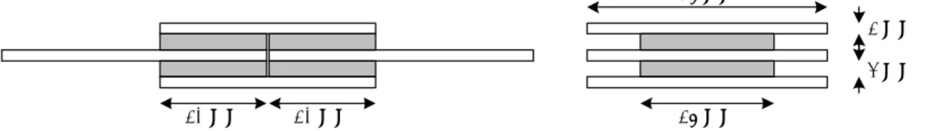
suppliers. The double overlap joint geometry given in figure 2, was used within these
tests. For the adherend an aluminium 6061-T6 alloy was selected. The nominal value
of the bondline thickness is equal to 3 mm and the area of one bondline is equal to
20·25 = 500 mm
2. Compared to the mostly used single lap joint the selected geometry
has several advantages. Due to its symmetry there is no non-linear bending effect as
in most practical applications. The extended width of the specimen makes it possible
to get the bondline thickness within a narrow scatterband. Another advantage of using
this specimen for the creep tests is that four bondlines are tested instead of one; the
creep results represent mean values.
20 mm 20 mm 25 mm 45 mm
2 mm 3 mm
Figure 2 - Selected geometry of specimen
The specimens were prepared and bonded according to the specification of the suppliers. After bonding the specimens were fixed and placed into a climate chamber (21 ºC, 50% RH) for 3 weeks.
Each creep test was performed under static circumstances. In total four different long- term load levels (average stresses equal to 0.1, 0.35, 0.5 and 0.8 MPa), two
temperatures (23 and 60 ºC) and a constant humidity (equal to 60 % RH) were considered. The long-term loads were applied by springs and the environmental circumstances were guaranteed by placing the test rig within a controlled climate chamber. For each situation one specimen was tested.
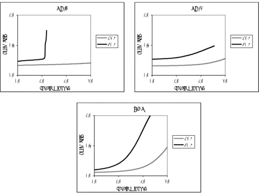
For each test the time-displacement curve was recorded. In figure 3 the results of three adhesives (two PU-formulations and one SMP-formulation) used in the same application, are presented for 23 ºC. The horizontal axis represents the log(10)-value of the loading time given in hours and the vertical axis represents the measured shear strain. The shear strain is defined as the displacement of one bondline divided by the bondline thickness. For a stress level of 0.1 MPa the creep curves for 23 ºC are compared in figure 4 with those for 60 ºC.
Based on these results the following observations are drawn. Initially the SMP-
formulation shows the lowest shear strain due to the applied stress level, but in time
the change in shear strain due to creep becomes more significant for the SMP-
formulation. At the lowest stress level (0.1 MPa) the change in shear strain due to
creep is much less for both PU-formulations, but at higher stress levels failure occurs
for the second PU-formulation within a shorter time period. The effect of a higher
constant temperature is not only restricted to an increase of the observed shear strains
for all three adhesives, but does also tend to initiate failure at an earlier stage.
0.1 MPa
0.0 0.2 0.4
0.0 1.0 2.0 3.0
log-time [hour]
shear strain PU-2
PU-1 SMP
0.35 MPa
0.0 0.5 1.0
-1.0 0.0 1.0 2.0
log-time [hour]
shear strain PU-2
PU-1 SMP
0.5 MPa
0.0 0.5 1.0 1.5 2.0
-1.0 0.0 1.0 2.0
log time [hour]
shear strain PU-2
PU-1 SMP
0.8 MPa
0 0.5 1 1.5 2
-1.5 -0.5 0.5 1.5
log-time [hour]
shear strain PU-2
PU-1 SMP
Figure 3 - Comparison of creep curves (time versus shear strain) determined for 23 ºC
SMP
0.0 0.5 1.0
0.0 1.0 2.0 3.0
log-time [hour]
shear strain 23 C
60 C PU-1
0.0 0.5 1.0
0.0 1.0 2.0 3.0
log-time [hour]
shear strain 23 C
60 C PU-2
0.0 0.5 1.0
0.0 1.0 2.0 3.0
log-time [hour]
shear strain 23 C
60 C
Figure 4 - Influence of temperature on creep curves for a stress level of 0.1 MPa
3 Empirical prediction model
To predict the creep at various stress levels, the shear strain rate has to be determined on basis of the time-shear strain creep curves as presented in figures 3 and 4. This shear strain rate is defined as:
) ( log t
g & = g (1)
Its value is constant during the stable creep period (after applying the long-term load and before excessive creep occurs) and can be determined mathematically from the time-shear strain curve.
To make an interpolation and extrapolation of the shear strain rates for the considered stress levels possible, a suitable relationship has to be defined. Many researchers have proposed to use an exponential function for creep. A major disadvantage for such a curve is that for extrapolated stress levels near 0 MPa unrealistic creep values might occur. For this reason it is proposed to use a 2nd order polynomial function with the additional condition that at a stress of 0 MPa the shear strain rate must be equal to 0:
t t t
g & ( ) = a ×
2+ b × (2)
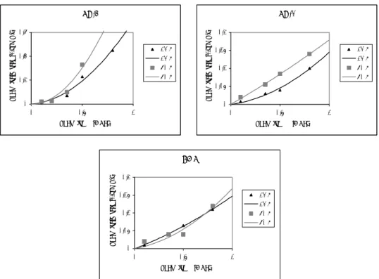
where g & ( t ) is the shear strain rate based on log(10) with the unit hours given as a function of the applied long-term shear stress τ with unit MPa. The constants a and b are determined by using a standard interpolation routine as for example incorporated within the program Excel. The results of this interpolation are presented in figure 5 for the three considered adhesives.
To apply these curve in practical engineering to predict the creep behaviour for a longer period of time (e.g. 10 years) the following remarks have to be considered:
- For practical applications the determined relationship might only be used for lower long-term stress levels (below 0.1 MPa). This is because the
interpolated data is based on the stable creep observed. For higher long-term stress levels the actual creep curves from tests should be used, which also takes into account unstable creep behaviour resulting into final failure.
- Each curve presented in figure 5 represents the mean value of test results of four specimens.
From figure 5 it can been seen that the test results for 60 ºC shows a higher
scatterband then the test results for 23 ºC. This will influence the accuracy of the
prediction for lower stress levels. Calculations show that for the SMP-adhesive (see
figure 5) it is possible to predict for 60 ºC lower shears strains than for 23 ºC. This
does not have any physical meaning. To avoid this problem it is necessary to make
use of probabilistic methods as described in the following chapter.
SMP
0 0.05 0.1 0.15 0.2
0 0.5 1
shear stress [MPa]
shear strain rate [1/log(h)]
23 C 23 C 60 C 60 C
PU-1
0 0.05 0.1 0.15 0.2
0 0.5 1
shear stresss [MPa]
shear strain rate [1/log(h)]
23 C 23 C 60 C 60 C PU-2
0 0.2 0.4 0.6
0 0.5 1
shear stress [MPa]
shear strain rate [1/log(h)]
23 C 23 C 60 C 60 C
Figure 5 - Interpolation of constant shear strain rates for 23 and 60 ºC
4 Development of simple design rules
The empirical prediction model proposed in the preceding chapter represents the mean value of the results of creep tests on overlap joints loaded in shear. To determine the design value with a given reliability (safety) level, the determined curves have to be calibrated with use of the methodology generally described by Van Straalen [1]. A more detailed description of this calibration technique is given in his PhD-thesis [2].
The design value of the shear strain rate g& , which meets the required reliability level,
dis defined such that the probability P of having a more unfavourable value equals:
) ( ) (
P g & > & g
d= F ab (3)
where Φ(·) is the standard normal distribution function. The parameters α and β are known as the weight factor and the reliability index, which both represent the
reliability level to be reached. Long-term deformations due to creep are caused by the
effects of the permanent loads and quasi-permanent values of the variable loads. Since
deformations have to be considered as a serviceability limit state, a target reliability
index equal to β = 1.5 has to be reached, as recommended in Eurocode: Basis of
structural design [3]. In addition a value of α = -0.8 should be taken for the weighting
factor. This factor takes into account that a part of the reliability is taken into account
As explained by Van Straalen [2], the design curve for the empirical relationship is based on the correction of the mean curve given by equation 2, by adding a factor K
d:
d 2
d
( t ) = a × t + b × t + K
g & (4)
To calculate the value of this factor K
d, the differences between the set of n test results and the matching calculated values of the prediction model have to be determined. For this set of correction factors K
ia normal distribution is assumed with a mean value K
mand a standard deviation K
s. According to Van Straalen [2] the design value is determined by the following relation:
K n t
K
K 1
1 )
(
sαβ m
d
= + n × × +
where t
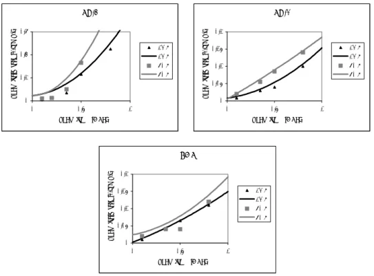
αβ(ν) is the value of the statistically known Student distribution with ν = n-1 degrees of freedom. Based on this procedure the design curves are calculated; in figure 6 these design curves are compared with the test results. From this comparison it is concluded that a larger scatter as for the 60 ºC curves, results in more
unfavourable design curves, which is the case for the lower shear stresses occurring in practice. For this reason it is recommended to perform more creep tests with lower values of the applied stresses.
SMP
0 0.05 0.1 0.15 0.2
0 0.5 1
shear stress [MPa]
shear strain rate [1/log(h)]
23 C 23 C 60 C 60 C
PU-1
0 0.05 0.1 0.15 0.2
0 0.5 1
shear stress [MPa]
shear strain rate [1/log(h)]
23 C 23 C 60 C 60 C PU-2
0 0.2 0.4 0.6
0 0.5 1
shear stress [MPa]
shear strain rate [1/log(h)]
23 C 23 C 60 C 60 C
Figure 6 - Comparison design curves for 23 and 60 ºC
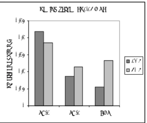
design values at 0.05 MPa
0 0.05 0.1 0.15 0.2 0.25
PU-1 PU-2 SMP
displacement [mm]
23 C 60 C
Figure 7 - Predicted displacement with a constant shear stress of 0.05 MPa for 10 years of loading
5 Development of an analytical prediction model
For the description of the deformation of solid polymers and also of cured adhesives, numerous strategies have been developed in time. Well known are linear visco-elastic constitutive models that describe the behaviour of polymers at low stresses and deformations. Often these models only deliver an one-dimensional description of the material behaviour and/or for one deformation mode only. The same limitations are often found in non-linear visco-elastic constitutive models for somewhat higher stress levels and deformations. Other constitutive models focus only on the yield behaviour at high stresses and deformations. In recent years however, developments in
constitutive modelling have been made, that allow many of the mechanical properties of solid polymers to be incorporated into three-dimensional constitutive models capable of combining (large) elastic and plastic deformation and accounting for load rate, type of load, temperature and pressure effects.
One of these constitutive models, which is currently being developed further by TNO BCR, is based on a so-called “Leonov mode”, as described by Tervoort [4] and Timmermans [5]. A single Leonov mode is a Maxwell model employing a relaxation time that is dependent on an equivalent stress, proportional to the Von Mises stress. It also separates between (elastic) hydrostatic stress and (visco-elastic) deviatoric stress.
The effect of temperature and strain softening is also accounted for. Govaert et al [6]
made an addition for the effect of water absorption. The ability to model creep (time dependent failure) was shown by Peijs et al [7].
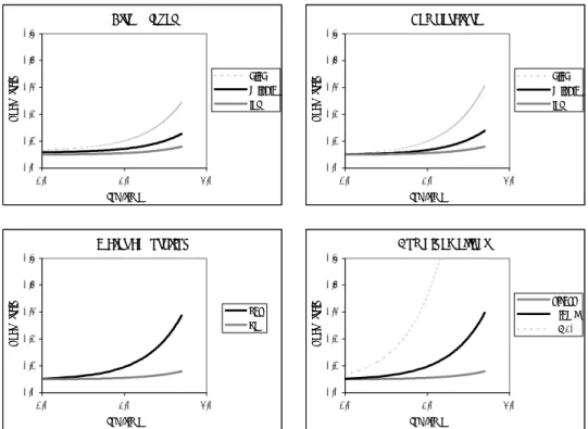
A mechanical analog of the model is shown in figure 8. By employing more Leonov modes in parallel (“multimode model”) more complex behaviour can be studied. The effect of strain hardening is incorporated by a single (3-D Neo-Hookean) spring [5].
Simulations of the influence of stress level, temperature, water absorption and
combined effects on the creep behaviour of adhesives are shown in figure 9.
Multiple Leonov modes
Strain hardening spring
Figure 8 – Mechanical analogue of constitutive model using multiple Leonov modes
Water absorption
0.0 0.1 0.2 0.3 0.4 0.5
1.0 2.0 3.0
log-time
shear strain
yes no
Temperature
0.0 0.1 0.2 0.3 0.4 0.5
1.0 2.0 3.0
log-time
shear strain high
middle low Stress level
0.0 0.1 0.2 0.3 0.4 0.5
1.0 2.0 3.0
log-time
shear strain high
middle low
Combined effects
0.0 0.1 0.2 0.3 0.4 0.5
1.0 2.0 3.0
log-time
shear strain stress
&temp
&H20