Quality grading of Hanwoo (Korean native cattle breed) sub-images using convolutional neural network

This is an Open Access article distributed under the terms of the Creative Commons Attribution Non-Commercial License (http: //creativecommons.org/licenses/by- nc/4.0/) which permits unrestricted non-commercial use, distribution, and reproduction in any medium, provided the original work is properly cited.

Copyright: © 2020 Korean Journal of Agrcultural Science

ANIMAL

Quality grading of Hanwoo (Korean native cattle breed) sub-images using convolutional neural network

Kyung-Do Kwon

, Ahyeong Lee

, Jongkuk Lim

, Soohyun Cho

, Wanghee Lee

, Byoung-Kwan Cho

, Youngwook Seo

1

National Institute of Agricultural Sciences, RDA, Wanju 55365, Korea

2

National Institute of Animal Sciences, RDA, Wanju 55365, Korea

3

Department of Biosystems Machinery Engineering, Chungnam National University, Daejeon 34134, Korea

*

Corresponding author: [email protected]

Abstract

The aim of this study was to develop a marbling classification and prediction model using small parts of sirloin images based on a deep learning algorithm, namely, a convolutional neural network (CNN). Samples were purchased from a commercial slaughterhouse in Korea, images for each grade were acquired, and the total images (n = 500) were assigned according to their grade number: 1++, 1+, 1, and both 2 & 3. The image acquisition system consists of a DSLR camera with a polarization filter to remove diffusive reflectance and two light sources (55 W). To correct the distorted original images, a radial correction algorithm was implemented. Color images of sirloins of Hanwoo (mixed with feeder cattle, steer, and calf) were divided and sub-images with image sizes of 161 × 161 were made to train the marbling prediction model. In this study, the convolutional neural network (CNN) has four convolution layers and yields prediction results in accordance with marbling grades (1++, 1+, 1, and 2&3). Every single layer uses a rectified linear unit (ReLU) function as an activation

function and max-pooling is used for extracting the edge between fat and muscle and reducing the variance of the data. Prediction accuracy was measured using an accuracy and kappa coefficient from a confusion matrix. We summed the prediction of sub-images and determined the total average prediction accuracy. Training accuracy was 100% and the test accuracy was 86%, indicating comparably good performance using the CNN. This study provides classification potential for predicting the marbling grade using color images and a convolutional neural network algorithm.

Keywords: beef marbling, convolutional neural network, deep learning, quality prediction, sub-images

OPEN ACCESS

Accepted: November 30, 2020 Revised: November 27, 2020 Received: August 25, 2020

Citation: Kwon KD, Lee A, Lim J, Cho S, Lee W, Cho BK, Seo Y. 2020. Quality grading of Hanwoo (Korean native cattle breed) sub- images using convolutional neural network.

Korean Journal of Agricultural Science 47:1109-1122. https://doi.org/10.7744/

kjoas.20200093

Introduction

Hanwoo cattle have been a native and major cattle breed in the Korean Peninsula since 3,000 B.C. (Lee et al., 2014). Four major breeds currently are commercial in Korea, and brown (Hanwoo) is the main domestic cattle breed for providing edible beef. Korean customers are prone to seeking tender, low-marbled meat, and thus the marbling index is an important factor in making consumption decisions of meat and its prices (Lee et al., 2017; Kang et al., 2019). Marbling in beef is relevant to the taste, tenderness, flavor, and juiciness (Platter et al., 2005).

In Korea, beef quality measurements are carried out by seeing the sirloin cut from between the 13th thoracic vertebrae and 1st lumbar vertebrae from the left half-carcass that has been kept in cold storage (- 4℃) for a day. There are five indices for deciding the beef quality: marbling index, muscle color, fat color, tenderness, and maturity. However, a number of inspectors still evaluate the quality grades using the standard card for decision color and marbling of beef without any equipment for acquiring scientific data to support their decision.

Currently, beef marbling and quality levels are determined by trained experts using beef marbling standard image cards, and thus the decisions depend on subjective, experienced visual assessments and environmental conditions such as lighting conditions or viewing angle (Sun et al., 2018). Since 2004, the beef marbling index in Korea has comprised nine beef marbling standards (BMSs), and their combinations yield five quality grades (QGs), 1++, 1+, 1, 2, and 3 (Gotoh and Joo, 2016). Among the 9 marbling BMSs, QG 3 includes BMS 1, QG 2 includes BMS 2 and 3, QG 1 includes BSM 4 and 5, QG 1+ includes BMS 6, and QG 1++ includes BMS 7, 8, and 9. Higher BMS beef contains more small and homogeneous fat

spreading on the sirloin.

Various computer vision-based approaches for the visual detection and grading of meat quality have been demonstrated such as image processing using a color camera (Farrow et al., 2009; Barbon et al., 2017), ultrasound (Greiner et al., 2003), and hyperspectral imaging (Pu et al., 2015; Wu et al., 2016). A quality comparison of fresh and frozen-thawed pork using hyperspectral imaging (Barbin et al., 2013; Ma et al., 2015; Pu et al., 2015) and frozen pork quality evaluation without thawing using a hyperspectral imaging system (Xie et al., 2015) have been reported. An artificial intelligence method (support vector machine, SVM) was also used to predict pork color and marbling (Sun et al., 2018). Furthermore, Barbon et al. (2017) reported the development of a computer vision system for beef marbling classification using the k-nearest neighbors (k-NN) algorithm.

Recently, image detection and classification algorithms have rapidly improved along with advancements in machine

learning, especially deep learning (DL) methods. DL convolutional algorithms have been successfully applied to classifying

image datasets (LeCun et al., 2015). Thus, so far, machine learning methods such as a convolutional neural network (CNN)

using ultrasound to analyse the intramuscular fat of pork (Kvam and Kongsro, 2017), classification of plant species (Dyrmann

et al., 2016), detection of plant disease (Mohanty et al., 2016), and food image recognition (Yanai and Kawano, 2015). Using

DL technique, the features can be detected and classified automatically on account of learning complex patterns of target

objects. However, to the best of our knowledge, DL has not yet been used as a classification method for beef marbling

based on color images. Given this, the present work aimed to develop a beef marbling measurement technique using a DL

algorithm and small pieces of color images. Image processing (image correction) and the CNN model applied to divide

images in the same area and develop a classification model, respectively.

Materials and Methods

Samples preparation

In Korea, beef quality is graded according to livestock product grading standards. The grading part on the left half-carcass is the cut on the sirloin side between the last thoracic vertebrae and the first lumbar vertebrae, including the longissimus muscle area. Samples evaluated by an inspection expert were purchased several times at a commercial slaughterhouse (Geonhwa Inc., Anseong, Korea) in 2017, and a total number of 100 of samples were prepared. Samples were stored in a refrigerator at 4℃ then took pictures at room temperature.

Image acquisition

The image acquisition system for beef images was composed of a light source, polarization filter, worktable, and RGB camera as shown in Fig. 1. The RGB camera (EOS 5Ds, CANON, Tokyo, Japan) contains a complementary metal-oxide semiconductor approximately 36 mm × 24 mm in size. The maximum effective number of pixels is approximately 50.6 million (8,688 × 5,792 pixels). The light source used for photographing (RB-5055-HF Lighting Unit, Kaiser Fototechnik, Buchen, GERMANY) consists of four 55 W fluorescent lamps, and the color temperature of the light source is 5,400 K.

To effectively remove the diffuse reflection generated during sample measurement, the RGB camera was equipped with a polarization filter (PR120-82, Midwest Optical Systems Inc., Palatine, USA) with a wavelength range of 400 to 700 nm and a contrast ratio of 10,000 : 1. In addition, the light source was also equipped with a polarization filter (HT008, Midwest Optical Systems Inc., Palatine, USA) with a contrast ratio of 10,000 : 1 in the range of 400 to 700 nm wavelength.

Image calibration for distortion correction

Radial distortion, a type of image distortion, occurs when the position of an object in an image is different from that in

real space (Park et al., 2009). Because this study considered fine intramuscular fat, even small parts of the image must be

positioned accurately, and thus distortion calibration of the sample images was required. Image distortion can be calculated

Fig. 1. Schematic design of the image acquisition devices for beef marbling classification with two light

sources.

and calibrated relatively simply, and the calibration of image distortion is widely used in research on image processing (Weng et al., 1992). Fig. 2 shows a schematic diagram of radial distortion in an image. Radial distortion occurs in the radial direction due to the deflection of light passing through the lens and defects in the lens, and depending on the type of distortion that occurs; it is classified into negative (barrel) distortion and positive (pincushion) distortion.

The proposed algorithm (Zhang, 2000; Lin et al., 2005; Park et al., 2009) was used to calibrate the radial distortion in the original images, and the distortion ratios were calibrated using the equation 1 and 2.

(1) (2)

In Eq. 1, X

, Y

are coordinates in the distorted image (b and c), and X

, Y

are coordinates in the calibrated image (a) in Fig. 3. If one point in the distorted image is P(X

, Y

) and one point in the distortion-calibrated image is P

( X

, Y

), by Eq.

1, the straight line distance (ΔR) between the difference in X-axis coordinates (ΔX) and difference in Y-axis coordinates ( ΔY) can be calculated. Since the ideal position is P', the distortion ratio is calculated by Eq. 2. A variety of open sources is commonly used for calibrating radial distortion. In this study, the single camera calibration toolbox (MATLAB R2016a, The MathWorks, Natick, USA) was used to calibrate radial distortion in the original images.

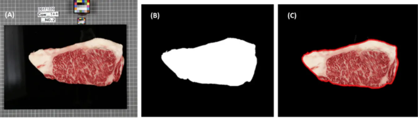
Image data preparation for analysis

In this study, we extracted only the region corresponding to the actual beef as the region of interest (ROI) from the area

that was calibrated for radial distortion and used it as the dataset. The size of the extracted ROI images varied slightly from

sample to sample but was approximately between 2,000 × 1,000 and 3,500 × 1,500 pixels, which is greatly reduced

compared with the initial image size (8,688 × 5,792 pixels). However, for the ImageNet Large Scale Visual Recognition

Challenge (Russakovsky et al., 2015), the image size for the input dataset is 224 × 224 pixels (Krizhevsky et al., 2012), and

the image size of the input dataset used for handwritten digits was 28 × 28 pixels (Niu et al., 2012). That is, the extracted

ROI images were thought to be too large to be used as input data. In other words, it would take a long time to perform

Fig. 2. (a) Corrected image and (b) radial distortion examples such as barrel distortion and (c) pincushion

distortion.

learning using the as-extracted ROI images as input data, and thus a different strategy was required to perform deep learning with limited samples. In contrast, a reduced pixel image had taken as a sample for beef marbling grading is not considered as the best strategy for reliable detection and classification.

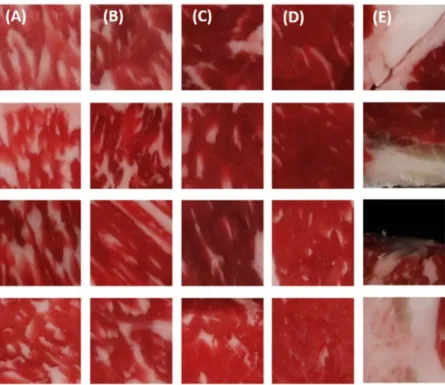
Therefore, we created a sub-image of 161 × 161 pixels and constructed a dataset that uses each sub-image as the input.

In our previous study, size of the sub-image for beef marbling grades, 161 × 161 pixels were the least and reasonable size among 28 and 161 pixels (Kwon et al., 2019).

According to the beef grade, there were 4 categories (1++, 1+, 1, and 2 & 3), the total training data comprised 1,200 images, the validation data comprised 210 images, and the test data comprised 88 images. Among the obtained beef samples, since the number of grade 2 and 3 images was much smaller than that of other grades, and these grades are not of much interest to consumers, this study set grade 2 and 3 images into one class of 2 & 3. In addition, for the training dataset, the number of images was increased to include left and right inversion and top and bottom inversion to address the overfitting problem and develop a high-performance CNN. In total, 3,600 images were used for training.

Finally, one image that was not used for training was prepared for each grade, and a sub-image of 161 × 161 pixels across the grading part was set as the prediction dataset. The results predicted from the complete grading area were checked. Based on this, the performance of the developed CNN was evaluated in comparison with the actual grading results.

Prediction model using CNN

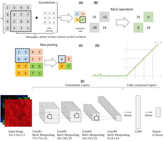
A CNN is an artificial neural network that creates the features of input images using various filters (kernels) to perform convolution operation, and learning is performed based on this. The features of input images are generated differently depending on filter size and stride, and different learning results are derived in accordance with each layer composition. In this study, we set the convolutional filter size to 3 × 3 which strides to 1 across the width and height of the input image and executes a dot product is computed to build up an activation map (Fig. 3A).

Primary algorithms used in the CNN configuration were ReLU (rectified linear unit), batch normalization, and dropout.

After the convolution operation, ReLU was used as the layer activation function (Fig. 3B and 3D). The use of ReLU function (f(x) = max(0,x)) enables learning with faster and higher performance than other activation functions such as logistic and hyperbolic tangent networks, and thus because it is widely used not only the image processing field but also in various study fields (Glorot et al., 2011).

To reduce computation time, the pooling process, known as downsampling, is applied to reduce the size of the image.

Currently, average and max-pooling are the most common methods, max-pooling layer consists of a sliding window function such as 2 × 2 that moves with stride 2 over the image matrix and gathers the highest number from the window. Max-pooling layer produces a new output matrix with the highest value from the original image matrix so that has the potential to stand out the edge of the image (Fig. 3C).

Batch size refers to the number of input data learned at a time. That is, even within a training process, the learning process

changes depending on the batch size. The batch normalization technique normalizes the results for each batch of input data

and uses the average in the test process. Batch normalization can be used to reduce covariate shifts and enables the design of

deeper layers (Ioffe and Szegedy, 2015).

Dropout, proposed by Srivastava et al. (2014), is involved in the activation of neurons in the corresponding layer and controls signal transmission to the next layer. This prevents overfitting and yields high-performance results through random dropping units include their connections during training.

The CNN architecture of this study, including the algorithms described above, is summarized in Fig. 3. There are four convolution layers and two fully-connected layers. A 3 × 3 kernel size of the max-pooling window and was used for subsampling in each convolution layer. ReLU was used as an activation function, and batch normalization was applied to all convolution layers.

Each fully-connected layer is connected to all neurons in the layer immediately preceding it. In the first fully-connected layer, 4,096 neurons of the preceding layer are connected to 1,000 neurons. The final fully-connected layer is connected to four categories, and the number of final outputs after the dropout is applied at a rate of 0.5. In this case, to solve a multi-class (4 grades of beef marbling) problem, softmax was used as the activation function.

In this study, Python (version 3.7.4) was used in the Ubuntu 16.04 version environment for CNN development and learning. The PC used for learning was equipped with a 2.6 GHz CPU (Intel core processor, Skylake, Intel Corporation, Santa Clara, USA) with 8 cores and 16 GB of RAM, and training for model took about 4 hours under this environment.

Fig. 3. The architecture of the convolutional neural network (CNN) structure for beef marbling classification

and prediction. (A) Convolution, (B) rectified linear unit (ReLU) operation layer, (C) max-pooling, (D) ReLU

function and (E) overall CNN architecture. The input image was trained through its 4 convolutional layers

and then outputs predicted probabilities between 0 and 1, represent 1 to 4 classes respectively, with the

threshold being 0.5 using softmax function.

Fig. 4. Radial distorted (A and C) image and corrected (B and D) image.

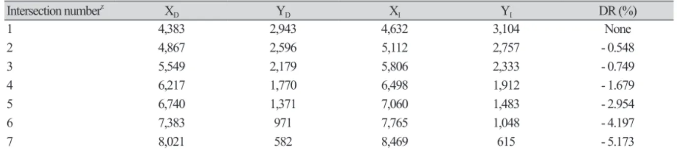
Table 1. Distortion ratio in accordance with intersection number from bottom left (1) to top right (7) of grid plate.

Intersection number

X

Y

X

Y

DR (%)

1 4,383 2,943 4,632 3,104 None

2 4,867 2,596 5,112 2,757 - 0.548

3 5,549 2,179 5,806 2,333 - 0.749

4 6,217 1,770 6,498 1,912 - 1.679

5 6,740 1,371 7,060 1,483 - 2.954

6 7,383 971 7,765 1,048 - 4.197

7 8,021 582 8,469 615 - 5.173

X

, X-axis coordinate of intersection point in a distorted image; Y

, Y-axis coordinate of intersection point in a distorted image; X

, X-axis coordinate of intersection point in a calibrated image; Y

, Y-axis coordinate of intersection point in a calibrated image; DR, distortion ratio.

z

Fig. 4C, 4D shows that yellow circles and numbers.

Results and Discussion

Image processing

The images before and after radial distortion calibration are shown in Fig. 4. Barrel distortion occurred in the original image (Fig. 4A), and in the calibrated image (Fig. 4B), it was confirmed that the lines forming the grid were calibrated. To examine the calibration quantitatively, the distortion ratio was calculated based on Equation 2. To obtain ΔX and ΔY required for the calculation of distortion ratio, the center point of the image and six grid intersections of the first quadrant were selected, which are shown as yellow circles in Fig. 4C and 4D. The center point of the image is labeled 1, the farthest point from the center point is labeled 7, and the coordinates and distortion ratio of each intersection point are summarized in Table 1.

The maximum value was observed with a - 5.17% distortion ratio at intersection point 7. The initial image size was 8,688

× 5,792 pixels, and thus 5.17% of the pixels on the x-axis correspond to approximately 449 pixels. Because of the large

amount of fine intramuscular fat in the image, it was thought that distorted 449 pixels could not be neglected. Therefore,

calibration of the radial distortion was necessary.

After specifying the rectangular area directly from the distortion-calibrated image, a sample image showed in Fig. 5A. The selected image was transformed to the grayscale (0 - 255) from the RGB color scale. A masking image was acquired by binarizing using threshold 25 as shown in Fig. 5B. The final ROI image (Fig. 5C) was extracted by multiplying the masking image and original image. Red-line on the selected ROI showed the acquired ROI was appropriate or not. In this way, the pre-processed images of all grades were set as ROI images.

Fig. 5. Image processing procedure to remove background and select region of interest (ROI) using mask. (A) Original image, (B) mask and (C) background removed image and selected ROI.

Sub-image for train

From the ROI images, we aimed to acquire a sub-image of 161 × 161 pixels as the initial experimental plan. Some images from the 3,600 datasets used for actual training were divided into four categories and are shown in Fig. 6. Although it varies depending on the image, the difference in the distributions of intramuscular fat between the categories is visible to the naked eye. However, not all sub-images could be used for learning. As shown in Fig. 6E, some mosaics included images that contained a large amount of fat or excess background, or images with an intramuscular fat distribution that was considered to not be representative of the corresponding grade. These images were excluded from learning. Nevertheless, the final goal is to develop a technique that can be applied to the entire grading part, and thus improvement is required. For the time being, the first improvement approach under consideration was to vary the sub-image sizes of 161 × 161 pixels. This is because as the size of the sub-image increases, it can serve as data that include the overall characteristics and not only a specific part inside the grading area. Another improvement method is to optimize the criteria for creating sub-images for each sample. Currently, the sub-image is generated at 161 × 161 pixels starting from the upper-left point of the ROI image. This can be changed to set an optimum point for each ROI image so that as much of the grading part is included as possible. Based on this method, it is necessary to optimize the sub-image technique to exclude parts that could cause errors.

The input data for prediction were one image for each grade, including all grading parts, and a total of four images were

extracted at 161 × 161 pixels. Sub-images were selected to include as much of the grading part as possible from the original

image. As a result of screening, 39 sub-images of grade 1++, 37 images of grade 1+, 44 images of grade 1, and 42 images of

grade 2 & 3 were identified. The sub-images for each grade screened in this way were used for prediction, and the screening

results are shown in Fig. 7. The sub-images contained inside the green line in each image were used for prediction.

Fig. 6. Sub-images of each quality grade. (A) is 1++ grade, (B) is 1+ grade, (C) is 1 grade, (D) is 2 & 3 grade and (E) is excluded parts for training and testing.

Fig. 7. Image mosaic and selected sub-images for model evaluation. Green outlines indicate model-applied

parts for each quality grade. (A) is 1++ grade, (B) is 1+ grade, (C) is 1 grade, and (D) is 2 & 3 grade.

Prediction model for marbling grade using CNN

The accuracy and loss for training and validation according to the learning epochs shows in Fig. 8. The best training and validation accuracies were 1.0 and 0.83, respectively. In 40 repetitions (epochs), the training accuracy approached at 1.0, and as the training was repeated until 100 epochs, the loss value tended to converge to zero. On the other hand, the accuracy and loss of validation did not change significantly and instead remained at constant values 0.83 and 0.48, respectively. This is thought to be due to the occurrence of overfitting despite using measures such as batch normalization, dropout, and increasing the learning data to reduce overfitting. The most important point is that the learning should proceed based on a larger dataset, and thus it is necessary to improve the learning time and hardware along with increasing the volume of data.

CNN classification results in a confusion matrix based on the test dataset in Fig. 9. For each of the 4 categories, 22 images were set as input data. In the test dataset prediction results, the highest performing category was grade 2 & 3 (100%).

The other three categories showed 81.8% accuracy, and the overall accuracy was 86%. Previous research for marbling classification using a computer vision system based on the k-NN method reported overall accuracy as 46.25, 78.34, and 81.59 which depends on the number of samples (n = 1 - 3) by different marbling scores based on human panel (Barbon et al., 2017).

The samples we used in this study were examining the results of the confusion matrix in detail, all four misclassifications generated from the input data of grade 1++ were classified as grade 1+, and four misclassifications generated from grade 1+ were classified as grade 1++. In addition, one misclassification at grade 1 was classified as grade 1+, and three were classified as grade 2 & 3. In other words, the prediction between adjacent grades was not accurately performed. Furthermore, as mentioned above, the input data are composed of 4 categories, not 5, which is the current quality grade system. Because of this problem, it is possible to classify the difference in the fine intramuscular fat distributions in the grade 2 & 3 images, ultimately, the development of an optimized CNN architecture is required to utilize small parts of the input data as features and classify them into 5 quality grades.

Fig. 8. (A) Accuracy and (B) loss of training (red line) and validation (black line) model for quality prediction

using convolutional neural network (CNN).

Fig. 9. Confusion matrix of test dataset with 22 sub-images for each quality grade class. The diagonal matrix represents the number of true positive among randomly selected 22 samples in parentheses.

Verification of the developed CNN model

The results of the prediction dataset showed as a confusion matrix in Fig. 10. Of the 39 total grade 1++ sub-images, 24 were predicted to be in grade 1++, 2 in grade 1+, 13 in grade 1, and 0 in grade 2 & 3 for a prediction accuracy of 61.54%. In other words, the quality inspector or consumers who want to know the quality grade of beef marbling can have prediction information such as 61.5% as 1++, 5% as 1+, 33.3% as 1 and 0% as grade 2 & 3.

Fig. 10. Confusion matrix of the convolutional neural network (CNN) model evaluation using one piece

of beef sample. The diagonal matrix represents the number of true positive among sub-part numbers (in

parentheses) extracted from one piece of each quality grade sample.

Of the 37 total grade 1+ sub-images, 18 were predicted to be in grade 1++, 15 were predicted to be in grade 1+, 4 were predicted to be in grade 1, and 0 were predicted to be in grade 2 & 3 for a prediction accuracy of 40.54%. Of the 44 total grade 1 sub-images, 0 were predicted to be in grade 1++, 2 were predicted to be in grade 1+, 28 were predicted to be in grade 1, and 14 were predicted to be in grade 2 & 3 for a prediction accuracy of 63.63%. Of the 42 total grade 2 & 3 sub-images, all were predicted to be grade 2 & 3 for a prediction accuracy of 100%. The total number of images used in the four categories was 162, with 109 correctly predicted, yielding an overall accuracy of 67.28%.

The prediction accuracy was found to be lower than the test accuracy in learning for all categories apart from the grade 2 & 3 images. It is thought that there were many misclassifications due to the difference between the existing grading methods, where a decision is made based on the overall grading part, and the method presented in this study, where one image is divided into sub- images of 161 × 161 pixels. As an example to illustrate this, a sub-image of grade 1++ was used as a prediction dataset, and parts of the image that were misclassified and their corresponding prediction results are shown in Fig. 11.

Fig. 11. Misclassified images for prediction results of 1++ grade.

The distribution of intramuscular fat in the images differs from the average grade 1++ intramuscular fat distribution as shown in previous Fig. 6. This shows that although this sample was determined to be grade 1++ when judged based on the overall grading part, depending on the position, some parts have different distributions of intramuscular fat than that of the determined grade (Barbon et al., 2017).

In future research, we intend to set the entire grading part as the input data to improve the above problem and consider the learning time and hardware configuration that will be required. In addition, since there are limits to the learning time and data acquisition, further investigation is required on the optimized size of sub-images representing the grading part.

Conclusion

In this study, we used a CNN for the objective classification of intramuscular fat, a major factor in beef grading. Four quality grading categories were used, and instead of the entire grading part, the CNN was developed with sub-images of 161

× 161 pixels. As a result, the training accuracy was 100% and the test accuracy was 86%, indicating a comparably good

performance which accuracy for marbling classification. However, there are limitations such as the small size of the obtained

dataset, limited hardware to utilize images requiring large capacity, lack of fully reflecting the current quality grading, and

a prediction accuracy that was lower than the test accuracy. Nonetheless, even with these limitations, the developed CNN

showed an accuracy of 67.28% for images of the grading part, and a further improvement in the predictive performance is

expected based on the difference in intramuscular fat distribution according to the position. Therefore, we plan to develop an

advanced classification model based on the CNN using sub-images developed in this study, and there is potential for using

the intramuscular fat as an objective indicator during the meat grading process and purchase by consumers.

Acknowledgements

This study was carried out with the support of �Research Program for Agricultural Science & Technology Development (PJ01181502) �.

Authors Information

Kyung-Do Kwon, https://orcid.org/0000-0003-2140-5333 Ahyeong Lee, https://orcid.org/0000-0002-8524-6282 Jongkuk Lim, https://orcid.org/0000-0002-2501-4367 Soohyun Cho, https://orcid.org/0000-0002-8073-8771 Wanghee Lee, https://orcid.org/0000-0002-8834-1779 Byoung-Kwan Cho, https://orcid.org/0000-0002-8397-9853 Youngwook Seo, https://orcid.org/0000-0003-2140-5333

References

Barbon AP, Barbon Jr S, Campos GF, Seixas Jr JL, Peres LM, Mastelini SM, Andreo N, Ulrici A, Bridi AM. 2017.

Development of a flexible computer vision system for marbling classification. Computers and Electronics in Agriculture 142:536-544.

Barbon DF, Sun DW, Su C. 2013. NIR hyperspectral imaging as non-destructive evaluation tool for the recognition of fresh and frozen–thawed porcine longissimus dorsi muscles. Innovative Food Science & Emerging Technologies 18:226-236.

Dyrmann M, Karstoft H, Midtiby HS. 2016. Plant species classification using deep convolutional neural network.

Biosystems Engineering 151:72-80.

Farrow RL, Loneragan GH, Pauli JW, Lawrence TE. 2009. An exploratory observational study to develop an improved method for quantifying beef carcass salable meat yield. Meat Science 82:143-150.

Glorot X, Bordes A, Bengio Y. 2011. Deep sparse rectifier neural networks. pp. 315-323. In Proceedings of the fourteenth international conference on artificial intelligence and statistics.

Gotoh T, Joo ST. 2016. Characteristics and health benefit of highly marbled Wagyu and Hanwoo beef. Korean Journal Food Science of Animal Resources 36:709-718.

Greiner SP, Rouse GH, Wilson DE, Cundiff LV, Wheeler TL. 2003. Prediction of retail product weight and percentage using ultrasound and carcass measurements in beef cattle. Journal of Animal Science 81:1736-1742.

Ioffe S, Szegedy C. 2015. Batch normalization: Accelerating deep network training by reducing internal covariate shift.

arXiv preprint arXiv:1502.03167.

Kang TH, Cho SK, Seo J, Kim M, Kim BW. 2019. Contribution analysis of carcass traits and seasonal effect on auction price for Hanwoo steers. Korean Journal of Agricultural Science 46:461-469. [in Korean]

Krizhevsky A, Sutskever I, Hinton GE. 2012. Imagenet classification with deep convolutional neural networks. pp. 1097- 1105. In Advances in Neural Information Processing Systems.

Kvam J, Kongsro J. 2017. In vivo prediction of intramuscular fat using ultrasound and deep learning. Computers and Electronics in Agriculture 142:521-523.

Kwon KD, Seo Y, Kim GY, Yoo HC, Lee WH, Cho BK. 2019. Feasibility study of convolutional neural network for beef

quality grade. p. 156. In Proceedings of the 2019 Spring Conference of Korean Society for Food Engineering.

Lee HJ, Choe J, Kim KT, Oh J, Lee DG, Kwon KM, Choi YI, Jo C. 2017. Analysis of low-marbled Hanwoo cow meat aged with different dry-aging methods. Asian-Australasian Journal of Animal Sciences 30:1733.

Lee SH, Park BH, Sharma A, Dang CG, Lee SS, Choi TJ, Choy YH, Kim HC, Jeon KJ, Kim SD, Yeon SH. 2014. Hanwoo cattle: Origin, domestication, breeding strategies and genomic selection. Journal of Animal Science and Technology 56:2.

Lin J, Sha D, Su D, Shen T. 2005. Distortion measurement of CCD imaging system with short focal length and large- field objective. Optics and Lasers in Engineering 43:1137-1144.

Ma J, Pu H, Sun DW, Gao W, Qu JH, Ma KY. 2015. Application of Vis–NIR hyperspectral imaging in classification between fresh and frozen-thawed pork Longissimus dorsi muscles. International Journal of refrigeration 50:10-18.

Mohanty SP, Hughes DP, Salathé M. 2016. Using deep learning for image-based plant disease detection. Frontiers in Plant Science 7:1419.

Niu XX, Suen CY. 2012. A novel hybrid CNN–SVM classifier for recognizing handwritten digits. Pattern Recognition 45:1318-1325.

Park J, Byun SC, Lee BU. 2009. Lens distortion correction using ideal image coordinates. IEEE Transactions on Consumer Electronics 55:987-991.

Platter WJ, Tatum JD, Belk KE, Koontz SR, Chapman PL, Smith GC. 2005. Effects of marbling and shear force on consumers' willingness to pay for beef strip loin steaks. Journal of Animal Science 83:890-899.

Pu H, Sun DW, Ma J, Cheng JH. 2015. Classification of fresh and frozen-thawed pork muscles using visible and near infrared hyperspectral imaging and textural analysis. Meat Science 99:81-88.

Russakovsky O, Deng J, Su H, Krause J, Satheesh S, Ma S, Huang Z, Karpathy A, Khosla A, Bernstein M, Berg AC. 2015.

Imagenet large scale visual recognition challenge. International Journal of Computer Vision 115:211-252.

Srivastava N, Hinton G, Krizhevsky A, Sutskever I, Salakhutdinov R. 2014. Dropout: A simple way to prevent neural networks from overfitting. The Journal of Machine Learning Research 15:1929-1958.

Sun X, Young J, Liu JH, Newman D. 2018. Prediction of pork loin quality using online computer vision system and artificial intelligence model. Meat Science 140:72-77.

Weng J, Cohen P, Herniou M. 1992. Camera calibration with distortion models and accuracy evaluation. IEEE Transactions on Pattern Analysis and Machine Intelligence 14:965-980.

Wu X, Song X, Qiu Z, He Y. 2016. Mapping of TBARS distribution in frozen-thawed port using NIR hyperspectral imaging.

Meat Science 113:92-96.

Xie A, Sun DW, Xu Z, Zhu Z. 2015. Rapid detection of frozen pork quality without thawing by Vis-NIR hyperspectral imaging technique. Talanta 139:208-215.

Yanai K, Kawano Y. 2015. Food image recognition using deep convolutional network with pre-training and fine-tuning.

pp. 1-6. In 2015 IEEE International Conference on Multimedia & Expo Workshops (ICMEW).

Zhang Z. 2000. A flexible new technique for camera calibration. IEEE Transactions on Pattern Analysis and Machine

Intelligence 22:1330-1334.