Multivariate Test based on the Multiple Testing Approach

Multivariate Test based on the Multiple Testing Approach

Seungman Hong

· Hyo-Il Park

1

Department of Informational Statistics, Korea University

2

Department of Statistics, Chongju University

(Received May 31, 2012; Revised July 25, 2012; Accepted September 13, 2012)

Abstract

In this study, we propose a new nonparametric test procedure for the multivariate data. In order to ac- commodate the generalized alternatives for the multivariate case, we construct test statistics via-values with some useful combining functions. Then we illustrate our procedure with an example and compare efficiency among the combining functions through a simulation study. Finally we discuss some interesting features related with the new nonparametric test as concluding remarks.

Keywords: Combining function, multivariate data, nonparametric test, permutation principle.

1. Introduction

To compare two populations with minimal assumption or assumptions for multivariate data, one may consider using one of nonparametric test procedures. The usual nonparametric test statistics have a quadratic form, which is a combining function and may be appropriate for testing the null hypothesis against the general type of alternatives. Puri and Sen (1971) have extensively studied and proposed multivariate nonparametric tests in this direction. However one may be interested in testing problems for the one-sided or ordered alternatives for the multivariate data. In this case, the quadratic form of test statistics may not be adequate for this purpose and several statisticians proposed nonparametric procedures with various approaches (Bhattacharyya and Johnson, 1970;

Boyett and Shuster, 1977). Also Park et al. (2001) proposed a nonparametric procedure for this problem by taking the maximum value among the standardized individual test statistics; however, one may consider to test hypotheses with combined types of alternatives. For example, for the bivariate case, one may be interested in the two-sided alternative for the first component or alter- natively a one-sided one for the second component and: however, (to the authors’ knowledge) any test procedure under this scheme for alternatives has not yet been proposed.

To obtain a critical value (or more generally a p-value) for any test statistics, we have to derive the null distribution (or at least limit the null distribution) for the statistics or combining functions.

This research was supported by the Korea University Research Fund.

2Corresponding author: Professor, Department of Statistics, Chongju University, Chongju 360-764, Korea.

E-mail: [email protected]

However, the derivation of the exact or limiting distributions would involve another derivation of covariances among the individual test statistics that may be difficult for some cases. Then it would be convenient to use the permutation principle (Fisher, 1925), which is a re-sampling method and requires enormous computational works. However, this has become the usual methodology in the applied areas of statistics with advanced computer facilities and relevant statistical software (cf.

Westfall and Young, 1993).

In this study, we propose a new nonparametric multivariate test procedure with the multiple testing approach for the generalized types of alternatives. In the next section, we begin our discussion by formulating generalized alternatives that may contain types of alternatives such as one- and two-sided for each component. Then we introduce three types of useful combining functions to construct test statistics via p-values. Then we illustrate our procedure with a numerical example and compare efficiency among the combining functions through a simulation study. Finally we discuss some interesting features related to our procedure.

2. Multivariate Test

Let X

, . . . , X

and Y

, . . . , Y

be two independent random samples from populations with d- variate distribution functions F and G, respectively. We assume the location translation model for the convenience of our formulation of the generalized alternatives. In the next section, we will briefly comment on the extension for the applications of our procedure other than the location translation model. Since we assume the location translation model, there is a d-dimensional real vector δ ∈ R

such that for all x ∈ R

,

G(x) = F (x − δ). (2.1)

Based on these samples and under the model (2.1), we assume that we are interested in testing H

: F = G or

H

: δ = 0. (2.2)

However, for the alternatives, we consider vary with component to component. Therefore for each i, i = 1, . . . , d, the alternative would be one of the following three forms:

H

: δ

̸= 0, H

: δ

> 0 and H

: δ

< 0, (2.3) where δ

is the i

component of δ ∈ R

. Then we may formulate the alternative corresponding to (2.2) as follows:

H

: ∪

H

. (2.4)

We note that in view of the expression (2.4) for the alternative, the null hypothesis in (2.2) can be rewritten as

H

: ∩

H

= ∩

{δ

= 0 } . (2.5)

Under this scheme of alternatives, first of all, we choose a suitable test procedure for each component

that can be parametric or nonparametric. Let λ

be the corresponding p-value for testing H

:

{δ

= 0} against any one of the three forms of alternatives in (2.3). In order to obtain an overall

p-value using these d number of λ

’s for each partial test, we have to choose a combining function

to combine the individual partial tests. In the following, we introduce useful combining functions

that have been used widely in applications (Pesarin, 2001).

(1) The Fisher omnibus combining function is based on the statistic

C

= −2

∑

log(λ

).

(2) Liptak combining function is based on the statistic

C

=

∑

Φ

(1 − λ

),

where Φ is the cumulative standard normal distribution function and Φ

, its inverse.

(3) The Tippett combining function is given by

C

= max {1 − λ

, . . . , 1 − λ

} .

In addition, one may consider using the quadratic form for a combining function; however, but the quadratic form is not suitable for the one-sided alternatives. Then we may reject H

for some large values of any one chosen combining function. To obtain an overall p-value, we need the null distribution for any chosen combining function; however, it would be difficult to obtain the null distribution of any C in the exact or asymptotic sense with the theoretic approach. For this reason, we may use the permutation principle. For the small sample case, we may obtain the exact null distribution of C and the resulting test has been known to be exact; however, for the large sample case (since it is difficult to consider all the configurations according to the permutation arguments even when the computer being used) it is common to apply the permutation principle with the Monte-Carlo approach. Then the result of the test would be asymptotic. Thus, we may complete this nonparametric test procedure by obtaining an overall p-value based on the exact or asymptotic permutation distribution.

For the application of the permutation principle for the multivariate case, it is important to under- stand that we have to permute the combined data with the observational-wise not the component- wise permutations. In this sense, we may have only (m + n)! permutations not [(m + n)!]

for the whole permutational configurations. Bell and Smith (1969) characterized this permutation principle in the multivariate case.

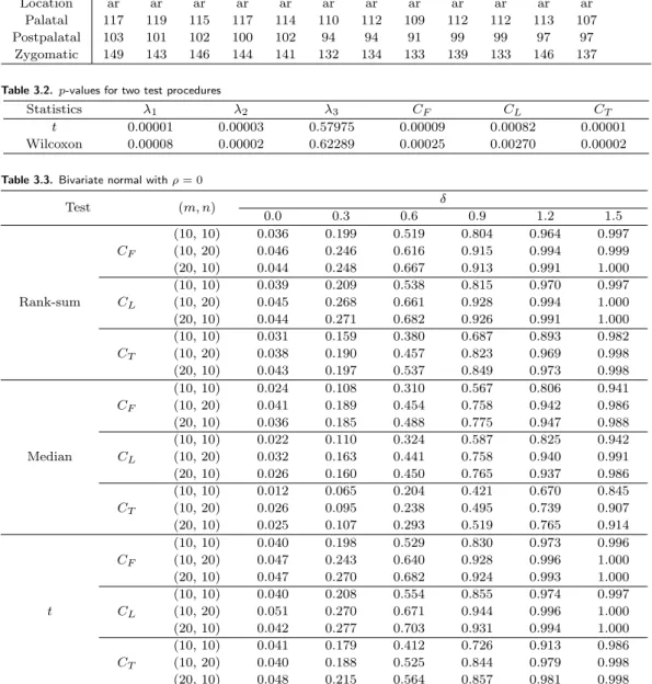
3. A Numerical Example, Simulation Results and Some Concluding Remarks

In order to illustrate our procedure, we consider the following data from Morrison (2004) on mea-

surements on the skull of the Eurasian wolf Canis Lupus L. For this study, we only considered

the first three characteristics(palatal and postpalatal lengths and zygomatic width) tabulated in

Table 3.1 to compare two wolf groups which are from rm(rocky mountain) and ac(arctic). We used

two kinds of test statistics for each individual test that are the two-sample t- and Wilcoxon rank

sum statistics for all characteristics with the three kinds of combining functions introduced in the

previous section. In order to obtain the individual p-values, we used the theoretical results and to

obtain the overall p-values, we used the permutation principle for both cases with the Monte-Carlo

method. The respective individual p-values and the overall p-values are tabulated in Table 3.2. In

this case, the t-tests yield more significant results and Tippett combining function(C

) produces

the most significant result among the combining functions.

Table 3.1. Canis L. data

No. 1 2 3 4 5 6 7 8 9 10 11 12 13

Location rm rm rm rm rm rm rm rm rm ar ar ar ar

Palatal 126 128 126 125 126 128 116 120 116 117 115 117 117

Postpalatal 104 111 108 109 107 110 102 103 103 99 100 106 101

Zygomatic 141 151 152 141 143 143 131 130 125 134 149 142 144

No. 14 15 16 17 18 19 20 21 22 23 24 25

Location ar ar ar ar ar ar ar ar ar ar ar ar

Palatal 117 119 115 117 114 110 112 109 112 112 113 107

Postpalatal 103 101 102 100 102 94 94 91 99 99 97 97

Zygomatic 149 143 146 144 141 132 134 133 139 133 146 137

Table 3.2. p-values for two test procedures

Statistics λ1 λ2 λ3 CF CL CT

t 0.00001 0.00003 0.57975 0.00009 0.00082 0.00001

Wilcoxon 0.00008 0.00002 0.62289 0.00025 0.00270 0.00002

Table 3.3. Bivariate normal with ρ = 0

Test (m, n) δ

0.0 0.3 0.6 0.9 1.2 1.5

(10, 10) 0.036 0.199 0.519 0.804 0.964 0.997

C_F (10, 20) 0.046 0.246 0.616 0.915 0.994 0.999

(20, 10) 0.044 0.248 0.667 0.913 0.991 1.000

(10, 10) 0.039 0.209 0.538 0.815 0.970 0.997

Rank-sum CL (10, 20) 0.045 0.268 0.661 0.928 0.994 1.000

(20, 10) 0.044 0.271 0.682 0.926 0.991 1.000

(10, 10) 0.031 0.159 0.380 0.687 0.893 0.982

CT (10, 20) 0.038 0.190 0.457 0.823 0.969 0.998

(20, 10) 0.043 0.197 0.537 0.849 0.973 0.998

(10, 10) 0.024 0.108 0.310 0.567 0.806 0.941

CF (10, 20) 0.041 0.189 0.454 0.758 0.942 0.986

(20, 10) 0.036 0.185 0.488 0.775 0.947 0.988

(10, 10) 0.022 0.110 0.324 0.587 0.825 0.942

Median C_L (10, 20) 0.032 0.163 0.441 0.758 0.940 0.991

(20, 10) 0.026 0.160 0.450 0.765 0.937 0.986

(10, 10) 0.012 0.065 0.204 0.421 0.670 0.845

CT (10, 20) 0.026 0.095 0.238 0.495 0.739 0.907

(20, 10) 0.025 0.107 0.293 0.519 0.765 0.914

(10, 10) 0.040 0.198 0.529 0.830 0.973 0.996

CF (10, 20) 0.047 0.243 0.640 0.928 0.996 1.000

(20, 10) 0.047 0.270 0.682 0.924 0.993 1.000

(10, 10) 0.040 0.208 0.554 0.855 0.974 0.997

t CL (10, 20) 0.051 0.270 0.671 0.944 0.996 1.000

(20, 10) 0.042 0.277 0.703 0.931 0.994 1.000

(10, 10) 0.041 0.179 0.412 0.726 0.913 0.986

C_T (10, 20) 0.040 0.188 0.525 0.844 0.979 0.998

(20, 10) 0.048 0.215 0.564 0.857 0.981 0.998

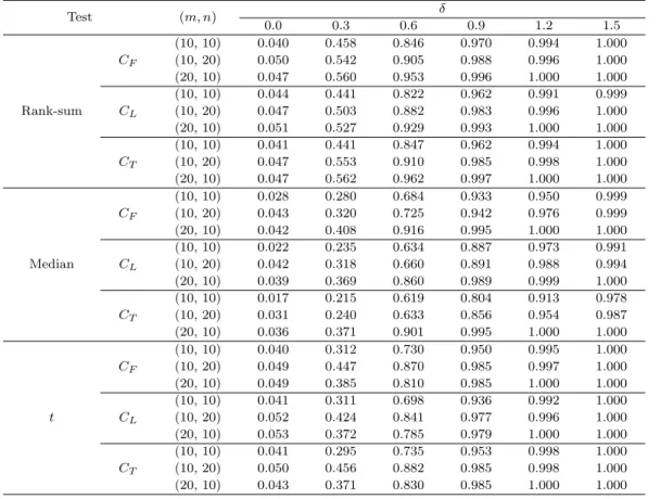
In order to compare the efficiency among the combining functions, C

, C

and C

, we have

conducted a simulation study. In this study, we obtained the empirical powers from the two types

of bivariate normal distributions and the Marshall-Olkin type of bivariate exponential distribution

Table 3.4. Bivariate normal with ρ = 1/2

Test (m, n) δ

0.0 0.3 0.6 0.9 1.2 1.5

(10, 10) 0.046 0.174 0.401 0.703 0.885 0.982

CF (10, 20) 0.043 0.200 0.499 0.826 0.960 0.997

(20, 10) 0.041 0.202 0.537 0.829 0.963 0.995

(10, 10) 0.045 0.178 0.399 0.702 0.886 0.979

Rank-sum CL (10, 20) 0.042 0.208 0.505 0.831 0.963 0.997

(20, 10) 0.040 0.205 0.543 0.828 0.962 0.995

(10, 10) 0.036 0.157 0.351 0.643 0.844 0.970

CT (10, 20) 0.040 0.179 0.439 0.770 0.937 0.993

(20, 10) 0.046 0.177 0.484 0.799 0.938 0.993

(10, 10) 0.026 0.113 0.268 0.508 0.751 0.905

CF (10, 20) 0.042 0.155 0.397 0.666 0.878 0.960

(20, 10) 0.034 0.146 0.393 0.659 0.874 0.969

(10, 10) 0.027 0.102 0.260 0.498 0.741 0.902

Median CL (10, 20) 0.038 0.145 0.366 0.658 0.872 0.967

(20, 10) 0.028 0.138 0.389 0.655 0.880 0.971

(10, 10) 0.016 0.067 0.189 0.383 0.621 0.806

CT (10, 20) 0.033 0.113 0.275 0.534 0.765 0.899

(20, 10) 0.027 0.111 0.314 0.540 0.757 0.964

(10, 10) 0.044 0.172 0.415 0.720 0.895 0.985

C_F (10, 20) 0.040 0.207 0.515 0.836 0.965 0.996

(20, 10) 0.046 0.207 0.552 0.840 0.964 0.997

(10, 10) 0.046 0.175 0.418 0.726 0.904 0.985

t CL (10, 20) 0.042 0.220 0.518 0.841 0.967 0.997

(20, 10) 0.040 0.208 0.551 0.841 0.967 0.997

(10, 10) 0.038 0.171 0.390 0.669 0.872 0.975

CT (10, 20) 0.043 0.185 0.485 0.787 0.955 0.995

(20, 10) 0.050 0.190 0.508 0.813 0.946 0.994

(Barlow and Proschan, 1975). For the bivariate normal distributions, one is independent, ρ = 0 and the other, dependent with ρ = 0.5 between two components. The pseudo random numbers for each component were generated with unit variance and the values of δ

, i = 1, 2, were varied from 0 to 1.5 by 0.3 increment for all distributions only with the case that δ

= δ

. The results are based on 1000 simulations and 2000 repetitions were carried out for each simulation to obtain the distributions for all combining functions using the permutation principle. The computations have been carried out by SAS/IML with PC version. The SAS program and various tips generating the pseudo random numbers for the multivariate normal distributions could be obtained from the internet. In addition, the readers may obtain the program upon the request from the authors. All the results are summarized in Table 3.3 to Table 3.5. The tests based on t show the most efficient performances for the normal distributions; however, the tests based on the Wilcoxon rank sum tests yield superb performances for the Marshall-Olkin type exponential distribution. The tests based on the median tests shows the inferiority for all cases. In addition, we note that C

obtains relatively low empirical powers among the three combining functions for all cases.

One may construct test statistics for testing (2.2) using directly the standardized form of statistics.

Then this approach cannot accommodate the alternatives in (2.3) with the combining functions

shown in the previous section. Therefore, this is a merit of our test procedure using the individual

p-values applied to the generalized alternatives.

Table 3.5. Marshall-Olkin type bivariate exponential

Test (m, n) δ

0.0 0.3 0.6 0.9 1.2 1.5

(10, 10) 0.040 0.458 0.846 0.970 0.994 1.000

CF (10, 20) 0.050 0.542 0.905 0.988 0.996 1.000

(20, 10) 0.047 0.560 0.953 0.996 1.000 1.000

(10, 10) 0.044 0.441 0.822 0.962 0.991 0.999

Rank-sum CL (10, 20) 0.047 0.503 0.882 0.983 0.996 1.000

(20, 10) 0.051 0.527 0.929 0.993 1.000 1.000

(10, 10) 0.041 0.441 0.847 0.962 0.994 1.000

CT (10, 20) 0.047 0.553 0.910 0.985 0.998 1.000

(20, 10) 0.047 0.562 0.962 0.997 1.000 1.000

(10, 10) 0.028 0.280 0.684 0.933 0.950 0.999

CF (10, 20) 0.043 0.320 0.725 0.942 0.976 0.999

(20, 10) 0.042 0.408 0.916 0.995 1.000 1.000

(10, 10) 0.022 0.235 0.634 0.887 0.973 0.991

Median CL (10, 20) 0.042 0.318 0.660 0.891 0.988 0.994

(20, 10) 0.039 0.369 0.860 0.989 0.999 1.000

(10, 10) 0.017 0.215 0.619 0.804 0.913 0.978

CT (10, 20) 0.031 0.240 0.633 0.856 0.954 0.987

(20, 10) 0.036 0.371 0.901 0.995 1.000 1.000

(10, 10) 0.040 0.312 0.730 0.950 0.995 1.000

C_F (10, 20) 0.049 0.447 0.870 0.985 0.997 1.000

(20, 10) 0.049 0.385 0.810 0.985 1.000 1.000

(10, 10) 0.041 0.311 0.698 0.936 0.992 1.000

t CL (10, 20) 0.052 0.424 0.841 0.977 0.996 1.000

(20, 10) 0.053 0.372 0.785 0.979 1.000 1.000

(10, 10) 0.041 0.295 0.735 0.953 0.998 1.000

CT (10, 20) 0.050 0.456 0.882 0.985 0.998 1.000

(20, 10) 0.043 0.371 0.830 0.985 1.000 1.000

In this paper, we only have confined ourselves to the location translation model. However since the constructions of test statistics were based on the individual p-values, we may extend the consider- ation for the applications of our procedure except for the location model (such as the scale) or the proportional hazards.

We note that we did not derive the null distribution or an asymptotic one of the combining functions because of the use of the permutation principle. This can be another merit of our procedure;

however, the required computational burden would be inexorably enormous if we additionally obtain the individual p-values with the permutation principle. Therefore it would be better to obtain the individual p-values with the theoretic approach and then apply the permutation principle to obtain the overall p-value.

It is also possible to use the bootstrap method (Efron, 1979; Shao and Tu, 1995) to obtain an

overall p-values, which is another re-sampling method. The difference between two methods are as

follows. The permutation principle resamples without replacement and the bootstrap method, with

replacement; however, sometimes the two methods yield quite different results (Good, 2000).

Acknowledgement

The authors wish to express their sincere appreciation to the referees for their constructive sugges- tions.

References

Barlow, R. E. and Proschan, F. (1975). Statistical Theory of Reliability and Life Testing, Probability Models, Holt, Rinehart and Winston, New York.

Bell, C. B. and Smith, P. J. (1969). Some Nonparametric Tests for the Multivariate Goodness-of-Fit, Multisample, Incomplete and Symmetry Problems, Multivariate Analysis, Ed. Krishnaiah, P. R., Academic Press.

Bhattacharyya, G. K. and Johnson, R. A. (1970). A layer rank test for ordered bivariate alternatives, Annals of Mathematical Statistics, 41, 1296–1310.

Boyett, J. M. and Shuster, J. J. (1977). Nonparametric one-sided tests in multivariate analysis with medical applications, Journal of American Statistical Association, 72, 665–668.

Efron, B. (1979). Bootstrap methods: Another look at the jackknife, Annals of Statistics, 7, 1–26.

Fisher, R. A. (1925). Statistical Methods for Research Workers, Oliver and Boyd, Edinburgh.

Good, P. (2000). Permutation Tests-A Practical Guide to Resampling Methods for Testing Hypotheses, 2nd Edition, Springer, New York.

Morrison, D. F. (2004). Multivariate Statistical Methods, 4th Edition. Thomson Brooks/Cole, New York.

Park, H. I., Na, J. H. and Desu, M. M. (2001). Nonparametric one-sided tests for multivariate data, Sankhya, Series B, 63, 286–297.

Pesarin, F. (2001). Multivariate Permutation Tests with Applications in Biostatistics, Wiley, New York.

Puri, M. L. and Sen, P. K. (1971). Nonparametric Methods in Multivariate Analysis, Wiley, New York.

Shao, J. and Tu, D. (1995). The Jackknife and Bootstrap, Springer, New York.

Westfall, P. H. and Young, S. S. (1993). Resampling-based Multiple Testing, Wiley, New York.