EVALUATION OF THE ATMOSPHERIC EFFECT FOR THE CLASSIFICATION USING HYPERSPECTRAL DATA
Sun-Hwa Kim, Jung-Il Shin, Hyung-Gap Cho, and Kyu-Sung Lee
Inha University, Department of Geoinformatic Engineering 253 Yonghyung-dong Nam-gu, Incheon 401-751, Korea
ABSTRACT: Spectral signal of remote sensing sensor are affected by scattering or absorption by water vapour, aerosol and gases. For reducing the atmospheric effect, various atmospheric correction algorithms from simple empirical model to complex radiative transfer model are used in the multispectral and hyperspectral data. The atmospheric correction procedure is surely needed in the target detection using hyperspectral image because this detection is constructed with comparing field or lab-measured reflectance spectrums. However it has to consider that the atmospheric correction is needed surely in the classification of hyperspectral data without matching the spectral library.
We analyze the quantitative atmospheric effect for the classification of Hyperion data. For this analysis, we used Hyperion data acquired at July 3, 2001, the absolute atmospheric correction based MODTRAN model, and classified 25 classes using three classification methods (Spectral Angle Mapper, Maximum-likelihood classification, Minimum distance classification). In the quantitative analysis of the 1st, 2nd statistics, spectral separability, and classification accuracy of the original radiance and corrected reflectance, there are no improving results of atmospheric correction.
Although the effects of atmospheric correction are different at each class, spectral band, classification method, this correction is normalized or simplified the detail hyperspectral spectral information. In the further study, we will attempt more detail analysis about the atmospheric effects for various classes.
KEY WORDS: MODIS, Content Separation Wavelet fusion, Spatial, Spectral, Wavelet Transform Modulus Maxima
1. INTRODUCTION
Spectral signal detected on the satellites influenced the scattering and absorption by the atmospheric gases, aerosols, and water vapor(Song et al., 2001; Elmahboub, 2000; Teillet, 1986; Chandrasekhar, 1960). Some studies attempt the atmospheric correction for the pre-processing step before the classification and change detection(Song et al., 2001). The aim of the atmospheric correction is to reduce the noise caused by atmosphere and extract the spectral reflectance of various land covers (Mahiny and Turner, 2007; Song et al., 2001; Holm et al., 1989).
Although there are many relative and absolute atmospheric corrections, it is not shown the noticeable improvement on the land cover classification or change detection. This phenomenon is caused that the atmospheric effect on the various land covers is different and the results are different from the atmospheric correction algorithm and classification methods. This study aims to evaluate and analyze quantitatively the atmospheric effect in the land cover classification using the hyperspectral image.
2. DATASET USED
Hyperspectral data provided a lot of spectral information as spectral library. For atmospheric correction, hyperspectral data provided the accurate and full reflectance spectrum using water vapor or carbon dioxide information extracted from hyperspectral image itself. The atmospheric correction proceeding is necessary to process hyperspectral data comparing with the multispectral data. This study used Hyperion data acquired on 3 June 3, 2001. Hyperion dataset is the satellite-borne hyperspectral data with 242 bands over 400~ 2,500nm wavelength region and has a spatial resolution of 30m. The study area is located in western part of central Korea and covers an area of about 10,000ha. Major land cover types of the study area are the forest, rice-paddy, and agricultural lands of several crop types. This study attempted to classify eight non- forest classes (quarry, water, grass, farm, etc.) and 17 forest classes divided by tree species, tree ages and topographic positions. Total 1803 training sites and 1802 test sites are used in this classification. For selecting training and test sites of cover type classes, we used aerial photographs of 1:15,000 scale acquired in May and October, 2001, the land use/cover maps of 1: 25,000 scale as the reference data. Additionally, forest maps of 1:25,000 and DEM dataset are used for classify the detail
forest cover types.
Figure1. Location of training and test samples (red : training sample, blue : test sample)
3. METHODS
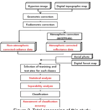
Figure 2 shows the total processing of this study. In this study, we used two Hyperion dataset that one is original radiance dataset and the other is the atmospheric corrected reflectance dataset. These two dataset are classified as three classification algorithms with same training sites. For evaluation of the atmospheric effects on hyperspectral data, we analyzed and compared quantitatively the 1st, 2nd statistics, separability, and classification accuracy of two Hyperion dataset.
Figure 2. Total processing of this study 3.1 Atmospheric correction method
For the atmospheric correction, we used FLAASH software based on MODTRAN radiative transfer code.
For more accurate correction, we used the water vapor
contents and carbon dioxide information extracted from Hyperion absorption bands as figure 3. These images provided the full atmospheric information at each pixel during image acquisition time. Additionally, this absolute atmospheric correction needed the input information as the average height, solar and sensor angle, geometric location, visibility, and atmospheric model. The atmospheric corrected reflectance image of Hyperion data is used for the land cover classification, and then compared with non-atmospheric corrected radiance image.
Figure 3. Water vapour image(left) and cloud mask image(right) calculated from Hyperion image and used in atmospheric correction of Hyperion image.
3.2 Classification method
This study applies three classification methods of minimum Euclidean distance(MED), maximum likelihood classification (MLC) and spectral angle mapper (SAM) to each image with or without atmospheric correction. Three classification algorithms used 1083 training sites for 25 land cover classes. While MLC and MED classification methods are the common classification algorithms, SAM algorithm is used the spectral angle between target signal for classification and signal defined for each class. The target or pixel for applying of classification algorithm is defined as the one class type showed the small spectral angle. After classification of two Hyperion dataset, we assessed the classification accuracy of each classes and total classes using 1,802 test sites.
3.3 Evaluation methods of the atmospheric effect The evaluation of the atmospheric effect is conducted by comparison of two Hyperion dataset with and without the atmospheric correction. First, the 1st statistics (mean, std., min/max, histogram) and 2nd statistics (correlation, coefficient of variation) of Hyperion dataset are comprised and analyzed. Second quantitative evaluation target is the separability between classes and spectral bands. For separability analysis, we used the Bhattacharyya distance and transformed divergence indices. Because this study focused on the effect of the atmospheric correction to the land cover classification, the classification accuracies of overall and each class are mainly evaluated.
4. RESULTS 4.1 Statistical analysis
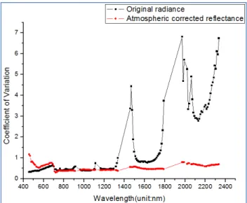
For comparing the radiance and reflectance with the different units, we analyzed the coefficient of variation.
As figure 4, there are the little differences at the visible wavelength near 400nm and large differences at the shortwave infrared wavelength area over 1300nm. At the standard absorption bands as gases and water vapor, it shows the largest difference between original radiance and atmospheric corrected reflectance. This difference is caused by the atmospheric correction at these absorption bands. Histograms of the radiance and reflectance show similar distribution pattern at standard wavelength area.
Figure 4. Coefficient of variation of Hyperion radiance and corrected reflectance.
As the 2st statistical analysis, we analyzed the correlation coefficient of radiance and reflectance as figure 5. Average correlation coefficient of the radiance (0.87) is little higher than the reflectance (0.77). At the correlation coefficient image of the reflectance, there are the large difference between visible, NIR, SWIR wavelength. As figure 5, the atmospheric corrected reflectance shows more normalized correlation coefficient than the Hyperion radiance data.
(a) (b)
Figure 5. Correlation image of Hyperion radiance(a), reflectance(b)
For more quantitative analysis, we analyzed the t-test results of the radiance and reflectance data as figure 6. At
figure 6, the major bands of Hyperion excepting 9 bands show the some differences between two correlation coefficients of radiance and reflectance.
Figure 6. T-test results between two correlation coefficients of Hyperion radiance and reflectance 4.2 Separability analysis
Table 1 shows the minimum and mean separability of Hyperion original radiance and atmospheric corrected reflectance image. Two separability indices are used as Bhattacharyya distance and transformed divergence. As Table I, Hyperion radiance image shows higher separability than reflectance image. Radiance image provides higher spectral separability between forest types (Chestnut-other forest types, Pine-Pinus Koraiensis, Deciduous-Mixed forest, etc…) than the reflectance image. The separability of the atmospheric corrected reflectance data shows lower or same separability value than original radiance data.
Table I. Minimum and mean separability using Bhattacharyya distance and Transformed Divergence of Hyperion radiance and atmospheric corrected reflectance image
Separ- ability
Bhattacharyya distance Transformed divergence Radiance Reflectance Radiance Reflectance Min 1.76 1.58 1,870 1,805 Mean 14.6 12.75 1,995 1,990
4.3 Classification accuracy
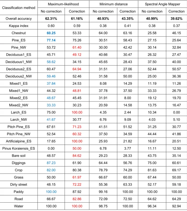
In the classification results, Hyperion original radiance and atmospheric corrected reflectance show similar accuracy. Among three classification algorithms, maximum-likelihood method is highest classification accuracy. Although overall classification accuracies of atmospheric corrected and non-corrected dataset are little low, the accuracy is higher excepting detail forest classes.
As table II, the accuracy of the reflectance image is little
Table II. Classification accuracy of atmospheric corrected and non-corrected hyperspectral image
higher than the radiance image on the bare soil, road, and dirty street. At the crop and diggings classes, the radiance data of no atmospheric correction shows higher than atmospheric corrected dataset. Because the forest classes have more complex structure and reflectance pattern, the accuracy or effect of the atmospheric correction in forest classes is not lower than other land covers. At other vegetation classes, the atmospheric correction doesn’t improve the accuracy of the land cover classification.
Although classification accuracy shows difference for three classification algorithms, atmospheric correction
doesn’t show the improvement of classification accuracy.
5. CONCLUSIONS
For analyzing hyperspectral data, the atmospheric correction is often regarded as a key processing step.
However, there are not many studies showing quantitatively the effect of atmospheric correction for the land cover classification. This study evaluated the effect of atmospheric correction for classifying 25 land cover types with EO-1 Hyperion data using various quantitative Classification method Maximum-likelihood Minimum distance Spectral Angle Mapper
No correction Correction No correction Correction No correction Correction Overall accuracy 62.31% 61.16% 40.93% 43.35% 40.99% 39.62%
Kappa index 0.60 0.59 0.38 0.41 0.38 0.37 Chestnut 60.25 53.33 64.00 63.16 25.58 46.15 Pine_ES 77.14 75.26 30.51 58.43 27.15 25.64 Pine_NW 53.72 61.40 30.00 42.42 30.14 32.84 Deciduous1_ES 45.71 49.12 40.66 30.47 26.32 27.47 Deciduous1_NW 58.62 34.15 45.65 28.43 37.50 40.00 Deciduous2_ES 60.47 64.94 31.51 27.06 52.44 50.57 Deciduous2_NW 59.46 52.46 31.58 50.00 25.00 36.36 Mixed1_ES 37.84 24.53 8.08 14.29 11.19 11.26 Mixed1_NW 44.32 48.81 37.78 37.50 33.33 26.79 Mixed2_ES 48.67 45.45 31.91 8.00 19.12 19.70 Mixed2_NW 33.33 30.23 20.59 14.58 13.75 16.47
Larch_ES 75.00 100.00 4.35 2.44 10.34 0.00 Larch_NW 41.67 30.77 6.76 9.09 4.03 5.10 Pitch Pine_ES 67.61 71.23 41.51 51.52 31.25 30.77 Pitch Pine_NW 52.54 60.32 37.50 34.59 44.44 41.86 Artificialpine_ES 17.65 100.00 25.93 21.82 16.67 20.51 Pinus Koraiensis_ES 0.00 50.00 6.78 3.77 11.11 12.50
Bare soil 48.57 84.62 29.23 28.33 43.75 35.14 Diggings 87.23 61.90 64.44 56.76 75.00 60.61 Crop 82.00 80.38 78.79 74.29 81.63 69.17 Grass 50.00 61.97 66.67 60.00 67.44 50.00 Dirty street 48.15 72.22 55.36 63.33 52.17 59.18 Paddy 100.00 87.92 99.16 100.00 100.00 100.00
Road 66.67 82.86 72.09 72.50 64.62 64.29 Water 100.00 100.00 98.75 100.00 96.34 92.94
indicators. In overall classification accuracy, the atmospheric corrected dataset did not show much improvement over the non-atmospheric corrected data.
The effects of atmospheric correction for land cover classification varied by land cover type. At detail forest classes having complex structure and various reflectance patterns, the effect of atmospheric correction is lower. In comparison of three classification algorithms, MLC was higher than SAM and MED algorithm. This study showed that the atmospheric correction may not be helpful for land cover classification with hyperspectral data. Further study is planned to analyze the more objective reason that the atmospheric correction didn’t show improvement of classification accuracy.
REFERENCES
[1] Chandrasekhar S., 1960. Radiative transfer, Dover, New York.
[2] Elmahboub W. M., 2000. A simulated linear mixture model to improve classification accuracy of satellite data utilizing degradation of atmospheric effect, Systemics, cybernetics and informatics, Vol.3(1):.25- 29.
[3] Holme R.G. et al., 1989. Surface reflectance factor retrieval from Thematic Mapper data, Remote Sensing of Environment, Vol.27: 717-725.
[4] Mahiny A. S. and Turner B.J., 2007. A comparison of four common atmospheric correction methods, Photogrammetric Engineering and Remote Sensing, Vol.73(4): 361-368.
[5] Song C. et al., 2001. Classification and change detection using Landat TM data: When and how to correct atmospheric effects?, Remote Sensing of Environment, 75:230-244
[6] Teillet P.M. et al., 2000. Landsat sensor cross- calibration using nearly-coincident matching scenes:
In Proceedings of the SPIE conference on Algorithms for multispectral, hyperspectral, and ultraspectral imagery VI, SPIE, Vol. 4049, Orlando, FL, in press.