1)
* 정회원, 한국건설기술연구원 선임연구원
** 정회원, 성균관대학교 토목공학과 부교수
2)
E-mail:[email protected] 031-910-0582
•본 논문에 대한 토의를 2002년 9월 30일까지 학회로 보내 주시면 2003년 1월호에 토론결과를 게재하겠습니다.
충격하중을 받는 박판의 후좌굴 해석
Postbuckling Analysis of Thin Plates under Impact Loading
김 형 열* 박 선 규**
Kim, Hyeong-Yeol Park, Sun-Kyu
Abstract
An explicit direct time integration method based solution algorithm is proposed to predict dynamic postbuckling response of thin plates. Based on the von Karman's plate equations and Marquerre's shallow shell theory, a rectangular plate finite element is formulated and utilized in this study. The element formulation takes into account geometrical nonlinearity and initial deflection of plates. The solution algorithm employs the central difference method.
Using the computer program developed by the authors, dynamic postbuckling behavior of elastic thin plates under impact loading is investigated by considering the time variation of load and load duration. The efficiency of the proposed solution algorithm is examined through illustrative numerical examples.
keywords : thin plate, finite element method, impact load, buckling, postbuckling, dynamic instability
요 지
Explicit 직접적분법을 사용하여 충격하중을 받는 박판의 후좌굴거동을 해석할 수 있는 알고리즘을 제안하 였다. von Karman의 대변위 판 이론과 Marquerre의 쉘 이론을 이용하여 유도한 직사각형 평판 유한요소 는 박판의 초기처짐과 기하학적 비선형 거동을 고려할 수 있다. 중앙차분법을 바탕으로 해석 알고리즘을 개발 하였고 이를 프로그램화 시켜, 하중형상과 재하시간이 다른 충격하중에 대하여 박판의 동적 좌굴거동을 해석 하였다. 수치해석 예제를 통하여 Explicit 직접적분법의 특성을 평가하였다.
핵심용어 : 박판, 유한요소법, 충격하중, 좌굴, 후좌굴, 동적좌굴, 초기처짐
1. INTRODUCTION
In recent years, due to the availability of high strength structural materials, many different types of thin-walled members have often been used as integrated parts of structures.
Thin-walled structural elements, when subjected to compressive stresses, are susceptible to buckling. In general, due to the postbuckling strength of plate elements, thin-walled members continue to resist stresses well above the local buckling stress. Since most elastic thin plates buckle at stresses well below the yield strength of the material, the inclusion of postbuckling strength in the design of thin-walled plate elements is economically essential.
The postbuckling analysis of plate elements is only possible through nonlinear analysis, which deals with the large deflection plate equations. In the finite element methods, mathematically complicated nonlinear equations are no longer intractable. Thus, a large number of finite element analysis procedures employing many different types of element have been developed for postbuckling analysis of plate elements.
Currently, most of the existing analysis procedures employ the load-deflection analysis procedure to determine postbuckling strength of plates (Gallagher et al. 1971).
In the existing postbuckling analysis procedures, dynamic loads are not generally considered as a part of the problem. In practice, however, thin-walled members are subjected to static as well as dynamic loads. It is commonly recognized that a structural compression member subjected to transient loads may undergo dynamic instability. In a certain circumstance, a suddenly applied transient load can cause buckling of
thin-walled compression members, even when its value is smaller than the static buckling load (Hoff 1967). Therefore, buckling analysis of plates often requires not only the determination of postbuckling strength, but a complete dynamic response of plates.
In this paper, postbuckling analysis of thin plates under impact loading is presented. The present study makes use of a rectangular plate element formulated by Kim (1997). The element formulation takes into account geometrical nonlinearity and initial deflection of plates. The explicit direct time integration method is utilized to overcome the difficulty in nonlinear transient analysis. Using the central difference method a computer code is developed, and its validity is verified through illustrative examples.
Dynamic postbuckling behavior of elastic thin plates under impact loading is investigated by considering the time variation of load and load duration. Dynamic loading parameters which play an important role in predicting the postbuckling response of thin plates are identified.
2 . DESCRIPTION OF SOLUTION METHOD
A general form of the differential equation of motion of an idealized structure can be semi-discretized using the finite element method with respect to space coordinates, and written in matrix form as (Bath 1982)
[ M] { D } + [ C] { D } + [ K] {D } = {Fex} (1)
where [M], [C], and [K] are the mass, damping, and stiffness matrices of the structure, respectively. {D} is the nodal displacement vector, and { D } and { D } are the corresponding nodal
velocity and acceleration vectors of the structure, respectively. {Fex} is a time dependent external force vector of the structure.
In order to reflect the time dependent nature of the problem, by denoting the current and previous time steps by t+△t and t, respectively, the semi-discretized matrix equations of motion in Eq. (1) can be rewritten as
[M] { D }t + Δt+ [ K] {D }t= {Fex}t + Δt (2)
It is noted that an arbitrary damping effect is excluded in the above expression. [M] is assumed to be time independent.
In the direct time integration methods, the space discretized matrix governing equation of a structure is solved by using either the implicit direct time integration method or the explicit direct time integration method (Bathe 1982). In the implicit method, the information at the current time step is obtained by iteratively adjusting the governing equation until internal and external equilibrium conditions are satisfied for that step. This method requires a great deal of additional computational effort in solving the simultaneous linear equations for every time step.
Whereas in the explicit method, the information at the current time step is obtained by directly solving the equation of motion at the previous time step. Hence, the solution of explicit method is obtained in a rather explicit and direct manner. It is noted, however, that a major drawback of the explicit method is in its inefficiency in inducing viable static solutions.
In explicit method of formulation, the element internal force vector can explicitly be calculated by (Cook et al. 1989)
{fin}t = ⌠
⌡V[ B]T{σ } dV (3)
where [B] is the element strain-displacement relation matrix, {σ} the element stress vector, and V the volume of the element. Hence, in explicit method, the governing matrix equation of the structural system in Eq. (2) can be rewritten as
[M] { D }t + Δt= {Fex}t + Δt- {Fin}t (4)
in which {Fin} is the internal force vector of the structure.
Knowing the structural external force vector at the current time step, the structural nodal acceleration vector can explicitly be computed as
{ D }t + Δt= [ M]- 1({Fex}t + Δt- {Fin}t) (5)
To obtain the solution, it is necessary to integrate Eq. (5) twice through the time space. The most commonly used operator in the explicit method is the central difference operator (Belytschko and Hsieh 1973). In this study, the equations of motion are integrated explicitly in time by the central difference method, in which the structural nodal velocity and displacement are computed as (Bath 1982)
{ D }t + Δt= { D }t+ 1
2 Δt[{ D }t+ { D }t + Δt] (6)
and
{D }t + Δt= {D }t+ Δt { D }t+ 1
2 Δt2{ D }t (7)
In the above, the structural nodal degrees of freedom are obtained without solving simultaneous equations, which is necessary in the implicit method. Since the structural stiffness matrix needs not be formed or stored, the explicit method can treat large scale problems with comparatively modest computer storage requirements.
In all cases of problems, the explicit method requires numerical integration along the loading path at high precision. Thus, many steps of numerical integration are always required.
Major disadvantage of the explicit method compared to the implicit method is that the explicit method requires very small time step for numerical stability requirements. Furthermore, {Fin} is needed to be recalculated at every time step even though the stiffness matrix is not changed. Therefore, the explicit method is suitable for only some special class of problems such as transient analysis of nonlinear problems.
3. FORMULATION OF ELEMENT EQUATIONS 3.1 Element Description
In this study, an isoparametric rectangular
plate finite element developed by Kim (1997) is reformulated using the explicit method of formulation. To be able to take into account geometrical nonlinearity and initial deflection of the plates, the element is formulated based on the von Karman's plate equations and Marquerre's shallow shell theory.
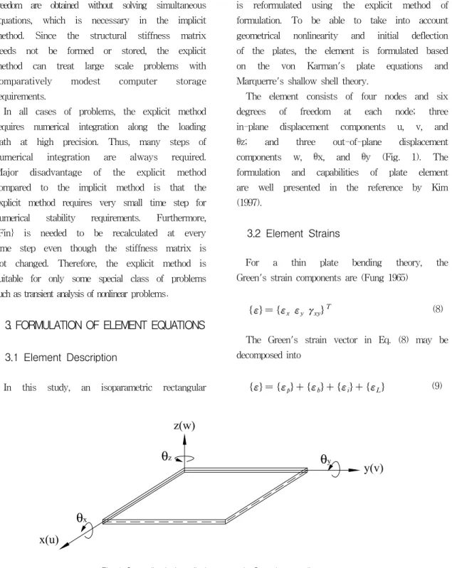
The element consists of four nodes and six degrees of freedom at each node; three in-plane displacement components u, v, and θz; and three out-of-plane displacement components w, θx, and θy (Fig. 1). The formulation and capabilities of plate element are well presented in the reference by Kim (1997).
3.2 Element Strains
For a thin plate bending theory, the Green's strain components are (Fung 1965)
{ε } = {εx εy γxy}T (8)
The Green's strain vector in Eq. (8) may be decomposed into
{ε } = {εp} + {εb} + {εi} + {εL} (9)
Fig. 1 Generalized plate displacements in Cartesian coordinates
z(w)
y(v)
x(u) θx
θy θz
where {εp} is the linear in-plane strain, {εb} is the bending strain due to the bending curvature of plate, {εi} is the linear contribution of the initial deflections to in-plane strain using Marquerre's strain expressions for shallow shells, and {εL} is the nonlinear large deflection strain.
Using the generalized kinematic relationships for plates, {εp} and {εb} can be determined, and given as
{εp} + {εb} = ꀊ
ꀖ ꀈ
︳︳
︳︳
︳︳
︳︳
︳︳
︳︳
∂uo
∂x
∂vo
∂y
∂uo
∂y + ∂vo
∂x ꀋ
ꀗ ꀉ
︳︳
︳︳
︳︳
︳︳
︳︳
︳︳ +
ꀊ
ꀖ ꀈ
︳︳
︳︳
︳︳
︳
︳︳
︳︳
︳︳
︳
- z ∂2wo
∂x2 -z ∂2wo
∂y2 -2z ∂2wo
∂x ∂y ꀋ
ꀗ ꀉ
︳︳
︳︳
︳︳
︳
︳︳
︳︳
︳︳
︳ (10a)
where uo, vo, and wo are the middle surface translations of the plate in the x, y, and z directions, respectively.
In Eq. (9), {εi} and {εL} can be determined using the von Karman's large deflection plate equations and Marquerre's strain expressions for shallow shells, and given as (von Karman et al. 1932, Marquerre 1938)
{εi} + {εL} = ꀊ
ꀖ ꀈ
︳︳
︳︳
︳︳
︳︳
︳︳
︳︳
∂wo
∂x
∂wi
∂x
∂wo
∂y
∂wi
∂y
∂wo
∂x
∂wi
∂y + ∂wi
∂x
∂wo
∂y ꀋ
ꀗ ꀉ
︳︳
︳︳
︳︳
︳︳
︳︳
︳︳
+ ꀊ
ꀖ ꀈ
︳︳
︳︳
︳︳
︳︳
︳︳
︳︳ 1
2( ∂w∂xo )2
1
2( ∂w∂yo )2
∂wo
∂x
∂wo
∂y ꀋ
ꀗ ꀉ
︳︳
︳︳
︳︳
︳︳
︳︳
︳︳
(10b)
where wi is the initial middle surface deflection of the plate in the z direction.
Using the relationships in Eqs. (10a) and (10b), and the shape functions presented in the reference by Kim (1997), generalized strain-displacement relation matrices [B] of the element can be constructed.
3.3 Element Stresses and Internal Force Vectors
In the implicit method of formulation, the geometrical nonlinearity is included in the nonlinear strain-displacement relations during the process of determining the tangent stiffness matrix. On the other hand, in the explicit method of formulation, this can be included efficiently during the process of determining the internal force vector without a great deal of additional computational effort.
In the following, the calculations of internal force vectors for the plate element are briefly presented.
In accordance with Eq. (9), matrices [B]
may be decomposed into
[ B ] = [ Bop
] + [ Bob
] + [ Bi] + [ BL] (11)
where [Bop] and [Bob] are the linear in-plane and bending related strain-displacement matrices, respectively. [Bi] and [BL] are the matrices that take into account the linear contribution of the initial deflection to the in-plane strain, and the change in geometry due to large deflection, respectively.
In the computer implementation, to avoid extensive zero multiplications, the element stress vector is separately calculated as
{σ } = {σop} + {σob} + {σL} (12)
where {σop} is the stress vector due to in-plane motion of the plate, {σob} the stress vector due to bending of the plate, and {σL}
the stress vector due to the initial deflections and the change in the geometry.
Using the element matrix [B] in Eq. (11) and the constitutive relationship for plates, each stress vector in Eq. (12) is respectively given by
{σop} = [ Dp][ Bpo] {di} (13a) {σob} = [ Dp][ Bbo] {do} (13b)
{σL} = [ Dp]([ Bi] + 12 [ BL]){do}(13c)
where [Dp] is the matrix containing the linear-elastic constitutive relationship for an elastic isotropic plate. {di} and {do} are the in-plane and out-of-plane nodal displacement vectors within the element, respectively, and given by
{di} = { uo vo θz}T (14a)
and
{do} = { wo θx θy}T (14b)
In the explicit method of formulation, the element internal force vector {fin} can be calculated by using Eq. (3). The element internal force vector due to the in-plane displacement, {fini}, is calculated as
{f iin} = ⌠⌡V [ Bpo]T ({σop} + {σL})dV (15a)
The element internal force vector due to the out-of-plane displacement, {fino}, is calculated as
{f oin} =
⌠⌡V([ Bbo]T{σob} + [ BL]T{σ L} + [ BL]T{σop})dV
(15b)
The integrations in Eqs. (15a) and (15b) must be integrated numerically. In the computer implementation, the Gaussian quadrature is employed for the numerical integration.
The internal force vector of the element, {fin}, is the sum of the two internal force vectors determined above, i.e.,
{fin} = {fin i} + {fin o} (16)
3.4 Element Mass Vector
A lumped mass matrix with the central difference method is a good combination in explicit methods (Cook et al. 1989). If the mass density and thickness within the element are constant, numerical integration with the 2x2 Gaussian quadrature rule is known to be sufficient. Since the lumped mass matrix is in the form of a diagonal matrix, all terms are merely vectors. In the computer implementation, the mass vector at the node i is calculated in the natural coordinates as
{mi} = ρt ⌠⌡ξ⌠
⌡η[ Ni]T[ Ni] ∣J ∣ dξdη (17)
where ρ is the mass density, t the thickness of element, and [Ni] the shape functions at node i. J is the determinant of the Jacobian matrix, which represents the area of the element, and ξ and η are the natural coordinates.
4. ILLUSTRATIVE NUMERICAL EXAMPLES
Using the reformulated plate element and central difference method, the solution algorithm is coded as the computer program. The validity of the computer program in predicting postbuckling response of thin plates under impact loadings is demonstrated through the example problems.
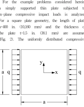
For the example problems considered herein, a simply supported thin plate subjected to in-plane compressive impact loads is analyzed.
For a square plate geometry, the length of plate a=400 in. (10,160 mm) and the thickness of the plate t=1.5 in. (38.1 mm) are assumed (Fig. 2). The uniformly distributed compressive
loads are applied in the x direction of the plate. In the analysis, one quarter of the plate is idealized using a 16 finite element mesh. For the material properties of the plate, an elastic modulus of 3.0x10⁷ psi (2.07x10⁵ MPa) and Poisson's ratio of 0.333 are assumed. Initial deflection of the plate is assumed to represent the locally buckled shape of the plate. For the simple support boundary condition, the initially deflected shape of the plate is represented by a double sinusoidal function for one quarter of the plate shown in Fig. 2 as
wi( x,y) = c cos πx
a cos πy
a (18)
where c is the maximum magnitude of initial imperfection of the plate. In the analysis, the maximum magnitude of initial imperfection is taken as c=0.1t. Due to the characteristics of the explicit method, the inertia force is required. For this example problem, the mass density of steel, ρ=7.35x10⁻⁴ lb-sec2/in4, is assumed. The shapes of load considered for the examples are the ramp and one half sine phase loadings (Fig. 3).
Fig. 3 Impulsive loadings: (a) ramp phase; (b) one half sine wave phase
Td t
P P
t Td
(a) (b)
Fig. 2 Geometry and loading conditions of square plate
x q y
a q
a
In the previous investigation for the dynamic instability problem (Kim 1996), the ramp, triangular, and one half sine shaped of impulsive loadings are considered. Since the shape of one half sine wave load is identified as a severe loading case, this shape is considered for the dynamic instability analysis. On the other hand, the ramp phase loading is utilized to induce the static behavior.
Gaussian numerical integration rule of 2x2 is used for the calculations of element mass and internal force vectors.
4.1 Plate under Pseudo-static Loading
Since the explicit method requires very small time step for numerical integration, this method is inefficient for static analysis.
However, for the purpose of comparison with the available analytical solutions, the static solutions are approximated using the pseudo-static loading. The uniform in-plane compressive loads of q/t=2247 psi (15.5 MPa) are applied at the middle surface of the plate in the x direction, as shown in Fig. 2. The load is increased using the predetermined loading rate of 7.5x10⁴ lb/sec. The time step used in the calculations is t=2.0x10⁻⁴ sec.
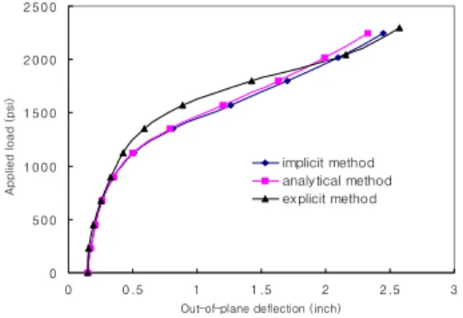
The applied load versus the maximum out-of-plane deflection of the plate is plotted in Fig. 4. In the figure, the obtained solutions are compared with the solutions obtained by the implicit method (Kim 1997) as well as analytical solutions by Williams and Walker (1977).
The solutions by the explicit method are smaller than those of both analytical and implicit methods until the load reaches q/t=2000 psi (13.8 MPa). This may be due to
the fact that the explicit method requires more times than the implicit method to reach the equilibrium because the explicit method does not perform iteration during the solution process. However, in the postbuckling range, the difference between three sets of solutions is negligible.
4.2 Plates under Impulsive Loading
The influence of impulsive loading on the dynamic postbuckling response of plate is briefly investigated. As shown in Fig. 3b, a one half sine shape of impulsive loading having various load durations is considered.
In the analysis, the magnitude of the impact load is unchanged, but durations of the load are changed to obtain the deflection versus time curves (histograms) for various load durations. The impact load has the maximum magnitude of q/t=2247 psi (15.5 MPa) at half the load. The duration of each load is normalized to the first period of free vibration of the unloaded plate. For this reason, the ratio of Td/Tn (the ratio between the period of the applied load and that of the first free vibration, Tn) is introduced.
Fig. 4 Comparison of solutions using the explicit method, implicit method, and analytical method
0 5 0 0 1 0 0 0 1 5 0 0 2 0 0 0 2 5 0 0
0 0 .5 1 1 .5 2 2 .5 3
Out-of-plane deflection (inch)
Applied load (psi)
implicit method analytical method explicit method
The natural frequency of the unloaded plate is ωn=14.01 rad/sec. Hence, the first duration of free vibration of the plate is Tn=0.4482 sec.
4.2.1 In-plane response of plate
In the first example, in-plane vibration of the plate due to impact loading is analyzed.
The maximum in-plane deflection at the plate edge under static loading is 0.0239 in. (0.607 mm).
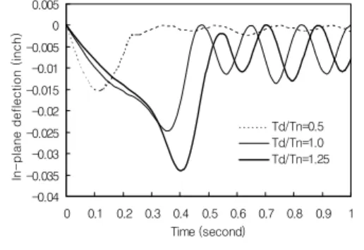
Fig. 5 shows the in-plane response curves for Td/Tn=0.5, 1.0, and 1.25, which correspond to load durations of 0.224 sec, 0.448 sec and 0.560 sec, respectively. The figure shows that the influence of load durations on the plate response is apparent. For the load duration of Td/Tn=1.25, the maximum in-plane response of the plate is 1.4 times larger than that of static loading. However, the influence of load durations on in-plane response of the plate is not severe.
4.2.2 Out-of-plane response of plate
In the second example, out-of-plane vibration of the plate induced by the in-plane impact
loading is investigated. The shape of the load and the duration of impact loading are the same as those in the previous example.
Fig. 6 shows the maximum out-of-plane deflection of the plate versus time curves for the load durations of Td/Tn=0.5, 1.0, and 1.25. For short load durations (Td/Tn<0.5), the dynamic effect is less than the static.
However, as the load duration increases, the dynamic effect becomes pronounced.
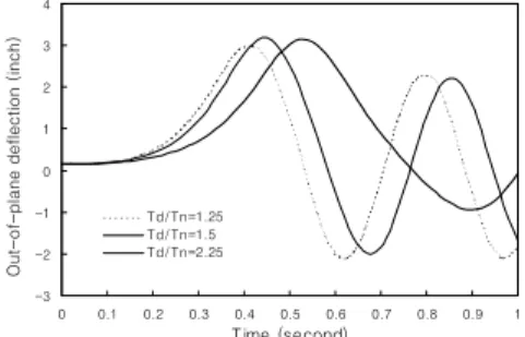
Fig. 7 shows the response of plates for which the values of Td/Tn are higher than unity. For relatively higher values of load duration (Td/Tn > 1.25), the amplitude of vibrations yields the deflections, which are 1.5 times larger than those of static loading. For a relatively long load duration (Td/Tn=1.25), the maximum out-of-plane amplitude is not further increased but the frequency of response is changed.
It is apparent that the dynamic postbuckling response of the plate is greatly influenced by the load duration. The results indicate that the value of Td/Tn=1.25 is assumed to be the critical value of dynamic instability for the plate under consideration.
Fig. 5 Influence of load durations on plate response (in-plane deflection versus time curves for Td/Tn=0.5, 1.0, and 1.25)
-0.04 -0.035 -0.03 -0.025 -0.02 -0.015 -0.01 -0.005 0 0.005
0 0.1 0.2 0.3 0.4 0.5 0.6 0.7 0.8 0.9 1 Time (second)
In-plane deflection (inch)
Td/Tn=0.5 Td/Tn=1.0 Td/Tn=1.25
Fig. 6 Influence of load durations on postbuckling response of plate (maximum out-of-plane deflection versus time curves for Td/Tn=0.5, 1.0, and 1.25)
-3 -2 -1 0 1 2 3 4
0 0.1 0.2 0.3 0.4 0.5 0.6 0.7 0.8 0.9 1
Time (second)
Out-of-plane deflection (inch)
Td/Tn=0.5 Td/Tn=1.0 Td/Tn=1.25
5. CONCLUSIONS
In this study, dynamic postbuckling behavior of thin plates under impulsive loadings is analyzed by using the explicit method. Based on the results of analysis for the selected example poblems, several conclusions can be drawn and are summarized in the followings.
1) The numerical results show that, for the plate postbuckling problems under short duration of transient loading, the explicit method is more efficient than the implicit method.
2) The results of example problems indicate that the dynamic postbuckling response of plates is greatly influenced by the load duration. For a short duration of impact load, the dynamic effect is less than the static effect. However, the influence of impulsive loading on postbuckling response is more pronounced as the load duration is increased.
3) For certain relationships between the load duration and the natural frequency of the plate, out-of-plane vibration occur with rapidly increasing amplitudes. Once the load duration reaches its critical value of
dynamic instability, the maximum dynamic response of the plate is about 50% larger than the corresponding static value.
4) The results of example problems have shown that dynamic postbuckling response of thin plates is quite different from the corresponding static response. It is therefore concluded that, where appropriate, the dynamic nature of loads must be considered in the structural problems to provide adequate safety against dynamic structural instability.
References
1. Bathe, K. J. (1982), Finite Element Procedures in Engineering Analysis, Prentice-Hall, Inc., N.J.
2. Belytschko, T. and Hsieh, B. T. (1973),
"Non-linear Transient Finite Element Analysis with Convected Coordinates," Int. J. Num.
Meth. Engr., 7, 255-271.
3. Cook, R. D., Malkus, D. S. and Plesha, M. E.
(1989), Concepts and Applications of Finite Element Analysis, 3rd Ed., John Wiley & Sons, Inc., New York, N.Y.
4. Fung, Y. C. (1965), Foundations of Solid Mechanics, Prentice-Hall, Inc., N.J.
5. Gallagher, R. H., Lien, S., and Mau, S. T.
(1971). "A procedure for finite element plate and pre-and post-buckling analysis." Proc., 3rd Conf. on Matrix Meth. in Str. Mech., Wright-Patterson Air Force Base, Ohio, 857-879.
6. Hoff, N. J. (1967), "Dynamic Stability of Structures," Proc. of Int. Conf. on Dynamic Stability of Structures, 7-41, Pergamon Press.
7. Kim, H. Y. (1996), "Dynamic Instability Analysis of Euler Column under Impact Loading,"
J. Computational Structural Engineering Institute of Korea, 9(3), 187-197.
8. Kim, H. Y. (1997), "Postbuckling Analysis of Geometrically Imperfect Plates by Finite Elements," J. of Str. Engr., KSCE, 17(I-4), 497-506.
Fig. 7 Influence of load durations on postbuckling response of plate (maximum out-of-plane deflection versus time curves for Td/Tn=0.25, 1.5, and 2.25)
-3 -2 -1 0 1 2 3 4
0 0.1 0.2 0.3 0.4 0.5 0.6 0.7 0.8 0.9 1
Time (second)
Out-of-plane deflection (inch)
Td/Tn=1.25 Td/Tn=1.5 Td/Tn=2.25
9. Marquerre, K. (1938), "Zur Theorie der Gekrummten Platte Grosser Formanderung."
Proc. of 5th Int. Cong. Appl. Mech., 93-101, John Wiley & Sons, Inc., New York, N.Y.
10. von Karman, T., Sechler, E. E., and Donnell, L. H. (1932). "The strength of thin plates in compression." Transaction, ASME., Vol. 54, 53-57.
11. Williams, D., and Walker, A. C. (1977),
"Explicit Solutions for Plate Buckling Analysis." J. Engr. Mech. Div., ASCE, 103(4), 549-568.
(접수일자 : 2002년 4월 29일)