The Analysis of Heat Transfer through the Multi-layered Wall of the Insulating Package

SCIENCE & TECHNOLOGY. Vol. 12, No. 1, 45~53 (2006) 45

The Analysis of Heat Transfer through the Multi-layered Wall of the Insulating Package

Seung-Jin Choi

School of Packaging, Michigan State University

Abstract Thermal insulation is used in a variety of applications to protect temperature sensitive products from thermal damage. Several factors affect the performance of insulation packages. Among these factors, the thermal resistance of the insulating wall is the most important factor to determine the performance of the insulating package. In many cases, insu- lating wall consists of multi-layered structure and the heat transfer through this structure is a very complex process. In this study, an one-dimensional mathematical model, which includes all of the heat transfer principles covering conduction, convection and radiation in multi-layered structure, were developed. Based on this model, several heat transfer phe- nomena occurred in the air space between the layer of the insulating wall were investigated. From the simulation results, it was observed that the heat transfer through the air space between the layer were dominated by conduction and radiation and the low emissivity of the surface of each solid layer of the wall can dramatically increase the thermal resistance of the wall. For practical use, an equation was derived for the calculation of the thermal resistance of a multi-layered wall.

Key words Thermal resistance, Insulating Package, Multi-layerd Wall

Introduction

Temperature sensitive products such as biological mate- rials, pharmaceuticals, industrial adhesives, gyroscopes, blood, frozen foods, fresh-products and dairy products should be shipped in temperature controlled containers which keep the temperature constant during transportation and keep products from thermal damage caused by melt- ing, thawing or freezing.

In most cases, thermal insulation is used to protect the products from thermal damage during distribution of prod- ucts. Thermal insulation is a procedure, which can retard heat transfer and eventually conserve energy by reducing heat loss or gain of the product (ASHRAE, 1993). Due to the complexity of the nature of heat transfer, several factors can affect the insulating ability of the containers.

The geometry of the package can affect the insulating capacity of the container. The addition of aluminum foil can also reduce the infrared radiation, which results sub- stantial improvement of the insulating ability of the pack- age. Sealing the package also plays important role for insulating ability of the package. Air currents can flow in and out through very small openings and can carry enough

heat with them to render even the best insulator ineffective.

Most of all, material’s resistance to heat penetration is the most crucial factor for the insulating ability of the package.

It is obvious that thicker walls generate better insulating capability. In many cases, multi-layered materials make better insulators than one thick material with the same thickness. A thin blanket of air trapped between the liner and box produces a significant resistance to heat pene- tration. This is the same principle behind double and triple pane windows or wearing layered clothes in the winter instead of one thick coat.

Because of the variety of factors affecting the perfor- mance of a thermally insulated package, a comprehensive model, which can represent these factors as much as pos- sible, is needed for designing efficient insulating packages.

Proper simulation model can reduce time-consuming efforts of preliminary specifications and subsequent val- idation tests. It also eliminates over-packaging and the resultant unnecessary costs. However, there were very few attempts to predict the ability of insulation packages (Bur- gess, 1999; Kositruangchai, 2003; Stavish, 1984). More- over, these models were over simplified or missed very crucial factors of heat transfer through insulating packages.

The first step to accomplish the comprehensive modelis to obtain an accurate thermal resistance of the wall of the insulating package. As mentioned above, material’s resis- tance to heat penetration is the most crucial factor for the insulating ability of the package. In this study, the math-

†Corresponding Author : Seung-Jin Choi

School of Packaging, Michigan State University, 130 Packaging Building, East Lansing, MI 48823, USA

E-mail : <[email protected]>

ematical model, which can predict the thermal resistance of the multi-layered wall, was developed.

If the wall consists of one material, it is very simple to calculate the thermal resistance of the package. For exam- ple, the thermal resistance of pure EPS is the reciprocal of its thermal conductivity, 0.038 W/m^.K. However, insulat- ing packages used in many applications employ much more complicated structures. Many insulating packages usea multi-layered structure with combinations of several insu- lating materials. In many cases, these layered materials are loosely fitted to each other to obtain extra thermal resis- tance by entrapping air between the insulating materials. A loose-fitting EPS foam jacket inside a corrugated box is a good example of these efforts. In this case, even though thermal conductivities of each of the insulating materials are known, it is still very difficult to estimate the overall thermal resistance of entire multi-layered structure because of the complexity of the heat transfer mechanisms through the ‘between the wall’air space.

To explain these phenomena and obtain an overall ther- mal resistance of the multi-layered insulating materials, all of the basic theories used in the previous part must be com- bined to yield a comprehensive mathematical model. For these reasons, a mathematical model of the wall by itself, not the entire package, was developed.

Theories

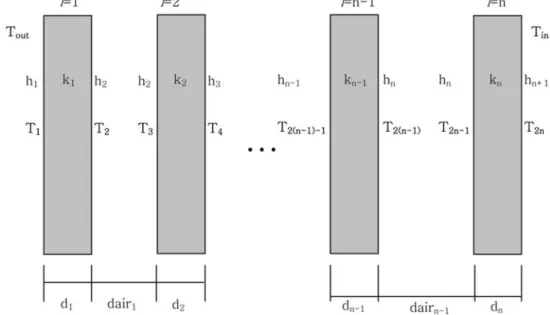
The one-dimensional diagram of a multi-layered wall is shown in Fig. 1. In this case, the area of the surface ofeach layer is the same all through the system. The heat can flow in both direction: from outside to inside or from inside to outside.

For convenience of the calculation, however, it is assumed that

the heat flows from outside to inside of the container.

In this diagram, the heat transfer through the wall occurs through the solid walls and air spaces between the wall.

The conduction heat transfer through i th layer can be described as

(1)

Q = heat transfer rate (W) A = cross-sectional area (m²)

k_i = conduction heat transfer coefficient (W/m^.K) T_2i-1, T_2i= temperature of the both side of i th layer (K) d_i = thickness of the i th layer (m)

The heat transfer through the air space between two walls is more complicated. In many practical problems, heat transfer through the air space can occur by three dis- tinct modes: conduction, convection and radiation. In this case, the total heat transfer where convection, conduction and radiation occur simultaneously can be described as:

(2)

h_i= h_r,i+ h_c,i (3)

h_i = effective convection heat transfer coefficient at i th air space (W/m^2.K)

h_r,i = radiation heat transfer coefficient at i th air space (W/m^2.K).

h_c,i= pure convection or pure conduction heat transfer coefficient at i th air space (W/m^2.K)

The radiation heat transfer rate between two parallel sur- Q

----A =k_i(T_2i–1–T_2i) d_i ---

Q

----A=h_i(T_2i–T_2i+1)

Fig. 1.Diagram of heat transfer through multi-layered wall in contact with inside and outside air

faces with same surface area can be described as the fol- lowing equation (Kreith, 1973):

(4)

σ = Boltsmann constant, 5.6×10⁻⁸ W/m^2.K⁴ ε2i, ε2i+1= surface emissivity of each side of the i th air

space

The pure convection or pure conduction heat transfer coef- ficient is determined by several factors (Holman, 1986): type of fluid (liquid or gas), flow condition (laminar or turbulent), forced or natural convection or phase change, free-stream velocity, surface geometry and roughness, position along the surface and temperature dependence of fluid properties.

This study deals with the heat transfer through the multi- wall structure. In this case, the conduction or convection in air space between the layers occurs in a confined air space.

In this study, only natural convection in confined air space was considered to represent convection heat transfer.

Natural convection heat transfer in enclosed spaces was investigated in various reports (Jacob, 1949; Kreith, 1973;

Holman, 1986). For an isothermal condition, the average natural convection heat transfer coefficient h_c,i in an enclosed air space between parallel planes can be expressed by the following empirical formulas:

(5)

k_i = thermal conductivity of air in i th air space (W/m^.K) dair_i = thickness of the i th air space (m)

Nu ₌Nusselt number in an enclosed air space.

Nusselt number is a strong function of Grashof number, Gr_δ, which is defined by

(6) ρ = density of air (Kg/m³)

γ = acceleration due to gravity (9.8 m/sec²)

β = volumetric coefficient of expansion of the air in (1/K)

∆Τ= positive temperature difference between the wall and the air in (K)

δ = thickness of the air space between the planes on either side (m)

µ = viscosity of air (Kg/m^.s)

Grashof number is important because when the Grashof number is below 2000, the heat transfer is dominated by conduction (Nu = 1.0) (Jacob, 1949 Kreith, 1973). When Grashof number is above 2000, the heat transfer is dom- inated by convection.

Using above heat transfer coefficients, the heat transfer

equations through the multi-layered structure can be derived. At steady state, the heat transfer rate through each solid layer is the same as the heat transfer rate through the air space between the solid layers. For an n layered wall with n-1 air spaces between them (See Fig. 1), one can establish a heat transfer balance with following equations assuming that all the area of the layered walls are the same.

for i = 1

(7) for i= 2 to n-1

(8) for i = n

(9) h_{r i,} σ ^T2i

4–T_2i+1⁴

( )/ T( _2i–T_2i+1) 1

ε2i

--- 1 ε2i+1

---–1 +

---

=

h_{c i,} k_i dair_i --- Nu⋅ _δ

=

Gr_δ ρ^2gβ∆^T′δ ³ µ² ---

=

Q

----A h₁(T_out–T₁) k₁ d₁

--- T( ₁–T₂) h= ₂

= (T₂–T₃)

=

h₁(T_{2 i( –1)}–T_2i–1) k_i d_i

= ----(T_2i–1–T_2i)hi+1+(T_2i–T_2i+1)

h₁(T_{2 n( –1)}–T_2n–1) k_n d_n ---

= (T_2n–1–T_2n) h= _n+1+(T_2n–T_in)

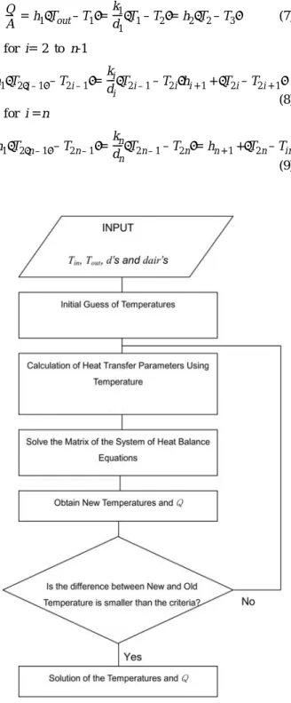
Fig. 2.Iteration procedure to solve non-linear problems.

d_i = thickness of the i th layer of solid material (m) dair_i= thickness of the i th layer of air space (m) k_i = conduction heat transfer coefficient of i th layer

of solid material (W/m^.K)

h_i = effective convection heat transfer coefficient for the i th air space from eq (3) (W/m^.K)

In this system of equations, there are 2N+1 unknowns (Q, T₁, T₂, …, T_2N-1, T_2N) and 2N+1 equations. However, this system of equations is highly non-linear. The con- vection and conduction coefficients, which are essential to solving for the unknown temperatures, are functions of the temperature itself. Moreover, radiation heat transfer coef- ficients include the terms of temperature powered by four.

To solve this non-linearity problem, an iterative procedure should be adopted to solve this problem. The diagram of this procedure is shown in Fig. 2.

Using this algorithm, the system of equations (7), (8) and (9) can be solved in terms of the heat transfer rate, Q, to yield (10)

In this case, the thermal resistance of the entire wall structure, R_wall, can be calculated as

R_wall= (11)

The unit of the Rwall is m^2.K/W.

Results and Discussion

1. Characteristics of the heat transfer in multi-lay- ered walls

One of the major questions about heat transfer within the airspaces in multi-layered walls is whether heat is con- ducted by conduction or by convection. In fact, this is determined by the Grashof number, Gr_δ, based on the thickness of the air space. As mentioned above, heat trans- fer is dominated by conduction if Gr_δ, is below 2000. Oth- erwise, heat transfer is dominated by convection.

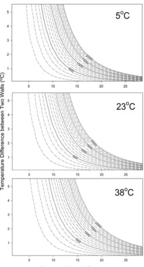
According to equation (6), Gr_δ, in confined space is a func- tion of the distance, δ, between the solid layers and the temperature difference between the layers, ∆T. The average temperature between the layers also affects Gr_δ, because ρ^2gβ^/µ² is a function of the average temperature between the layers. Using this equation, the characteristics of heat transfer of ‘between-the-wall’ air space was simulated.

The BASIC program NGR.BAS was constructed for simulation. Using this program, Gr_δ, was calculated with variety of δ^, ∆T and the average temperature of the wall. In most packaging applications, the distance between the two

solid layersis less than 20 mm and the temperature dif- ference between this thin air space is less than 5^oC. For these reasons, δ ^and ∆T were restricted 0.2 to 25 mm and 0.1 to 5^oC, respectively. Average temperatures of 5^oC, 23^oC, 38^oC were chosen to represent the low temperature, room temperature and high temperature, respectively. The simulation results are shown in Fig. 3 as a contour plot.

When Gr_δ, is higher than 2000, which is the upper right part of each graph, heat transfer is dominated by con- vection. When the distance between the solid walls is smaller than 13 mm (0.5 inch), heat is transferred mainly by conduction regardless of the temperature difference or the average temperature in the simulation range. In most cases, the thickness of the air spaces in multi-layered walls is very thin (< 10 mm). This means that the most of the heat transfer in ‘between the wall’ air spaces are dominated by conduction combined with radiation.

2. Development of the formula to calculate the R- value of multi-layered wall structure

From the simulation result in previous section, one can Q

----A T₁–T_n d_i k_i ----

i=1 n

∑

i=1 n–1

∑

+ ---

=

d_i k_i ----

i=1 n

∑

i=1 n–1

∑

+

Fig. 3.The Grashof number with the distance between the lay- ers and the temperature difference between the layers

assume that heat transfer in the air space is dominated by conduction and radiation. In this case, the effective heat transfer coefficient in equation (3) can be rearranged as

h_i= h_c,i+ h_r,i= (12)

Then, thermal resistance of a multi-layered wall in equa- tion (11) can be rearranged as

R_wall= T_solid+ R_air=

= (13)

In the equation(13), thermal resistance of the entire wall structure is composed of two main factors: the resistance from the solid material (R_solid) and the resistance of air space between the walls (R_air).

According to equation (4), the radiation heat transfer coef- ficient is a function of the emissivities of both surfaces. If one or both surfaces are foiled with aluminum, the radiation heat transfer coefficient, h_r,i, can be reduced dramatically. In this case, thermal resistance of the air space in equation (13) becomes a linear function of the distance between the walls over the conductivity of the air (dair/kair).

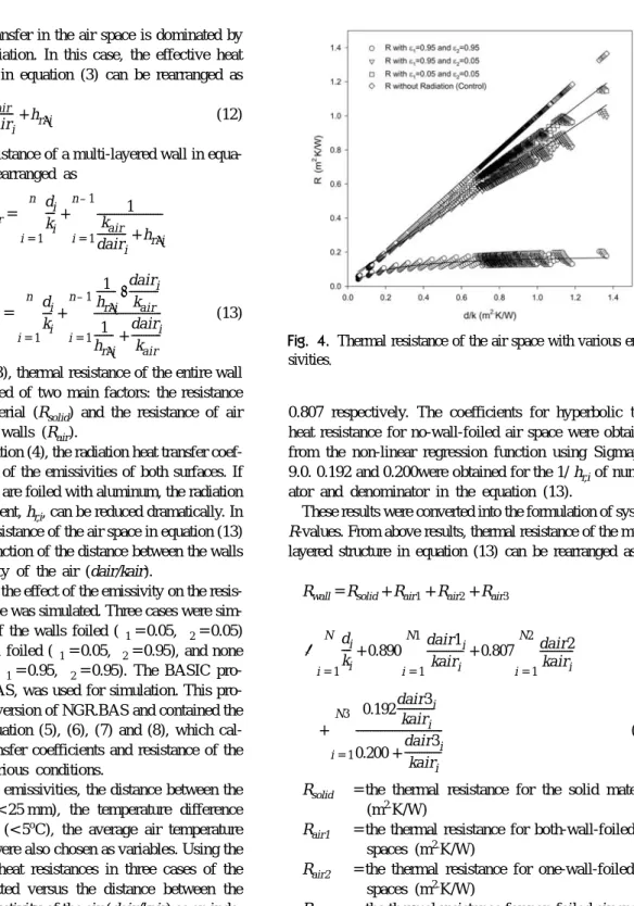
For these reasons, the effect of the emissivity on the resis- tance by the air space was simulated. Three cases were sim- ulated: both sides of the walls foiled (ε1= 0.05, ε2= 0.05) one side of the wall foiled (ε1= 0.05, ε2= 0.95), and none of the wall foiled (ε1= 0.95, ε2= 0.95). The BASIC pro- gram, NUSSELT.BAS, was used for simulation. This pro- gram is a modified version of NGR.BAS and contained the algorithm using equation (5), (6), (7) and (8), which cal- culates the heat transfer coefficients and resistance of the air space under various conditions.

In addition to the emissivities, the distance between the two solid layers (< 25 mm), the temperature difference between the layers (< 5^oC), the average air temperature (5^oC, 23^oC, 38^oC) were also chosen as variables. Using the simulation results, heat resistances in three cases of the radiation were plotted versus the distance between the walls over the conductivity of the air (dair/kair) as an inde- pendent variable.

As shown in Fig. 4, the three cases of radiation resulted in three distinctive patterns of resistance according to the independent variable, dair/kair. Moreover, the resistances of the air space showed a linear pattern when the emissivity of either walls is small (one or more walls are foiled). The resistances of the air space in these two cases were lin- earized as functions of dair/kair. Linear coefficients for the cases of two-walls- foiled and one-wall-foiled are 0.890and

0.807 respectively. The coefficients for hyperbolic type heat resistance for no-wall-foiled air space were obtained from the non-linear regression function using Sigmaplot 9.0. 0.192 and 0.200were obtained for the 1/ h_r,i of numer- ator and denominator in the equation (13).

These results were converted into the formulation of system R-values. From above results, thermal resistance of the multi- layered structure in equation (13) can be rearranged as

R_wall= R_solid+ R_air1+ R_air2+ R_air3

(14)

R_solid = the thermal resistance for the solid material (m^2.K/W)

R_air1 = the thermal resistance for both-wall-foiled air spaces (m^2.K/W)

R_air2 = the thermal resistance for one-wall-foiled air spaces (m^2.K/W)

R_air3 = the thermal resistance for non-foiled air spaces (m^2.K/W)

N = the number of solid layers

N₁ = the number of both-wall-foiled air spaces N₂ = the number of one-wall-foiled air spaces N₃ = the number of the airspaces without foiled layers d_i = the thickness of solid material of i th layer (m) dair1_i = the thickness of i th air space which has both-

wall-foiled surfaces (m)

dair2_i = the thickness of i th air space which has one- k_air

dair_i ---+h_{r i,}

d_i k_i

---- 1 k_air dair_i ---+h_{r i,} ---

i=1 n–1

∑

+

i=1

∑

d_i k_i ----

i=1

∑

1 h_{r i,} --- dair_i

k_air ---

⋅ 1 h_{r i,} --- dair_i

k_air --- + ---

i=1 n–1

∑

+

d_i k_i

----+0.890 dair1_i kair_i ---

i=1

∑

---

i=1

∑

∑

≅

0.192dair3_i kair_i ---

0.200 dair3_i kair_i --- + ---

i=1 N 3

∑

+

Fig. 4. Thermal resistance of the air space with various emis- sivities.

wall-foiled surfaces (m)

dair3_i = the thickness of the i th non-foiled air space (m)

Assuming that the conductivity of the solid material, k_i, is 0.038 W/m^.K, which is usually the case with insulating mate- rials, and the conductivity of the air, kair_i, is 0.028 W/m^.K, the resistance of the solid material in equation (14) can be described as:

R_wall= 0.026ths + 0.032tha1 + 0.029tha2 +

(15) ths = total thickness of solid layer (mm)

tha1 = total thickness of both-wall-foiled air space (mm) tha2 = total thickness of one-wall-foiled air space (mm) N₃ = number of the airspaces without foiled layer dair3_i = thickness of the i th non-foiled air space (mm)

3. Evaluation and refinement of the simplified equa- tion using computer program

In the previous section, a model was constructed to rep- resent heat transfer through a multi-layered wall structure.

The model was based on heat transfer theories, so it depends on the assumptions that could generate errors. For example, the model assumed that the conductivity of the air was constant at 0.028 W/m^.K. In the real world, however, the conductivity of air is a function of its temperature.

These kinds of errors should be minor ones, but they might accumulate and create huge disagreements between the model and real situations. For these reasons, evaluation and refinement of the model is necessary. To evaluatethe model, a computer program including all parameters which could affect heat transfer was constructed. BASIC program WALLBG7.BAS was constructed. 96 different cases of multi-layered walls were arbitrary chosen with various constructions (Choi, 2004). Using these data, WALLBG7.

BAS created R-values, total thickness of solid layers, total thickness of both-wall-foiled layers, total thickness of one- side-foiled layers, the number of the airspaces without foiled layers and the thickness of each non-foiled air space.

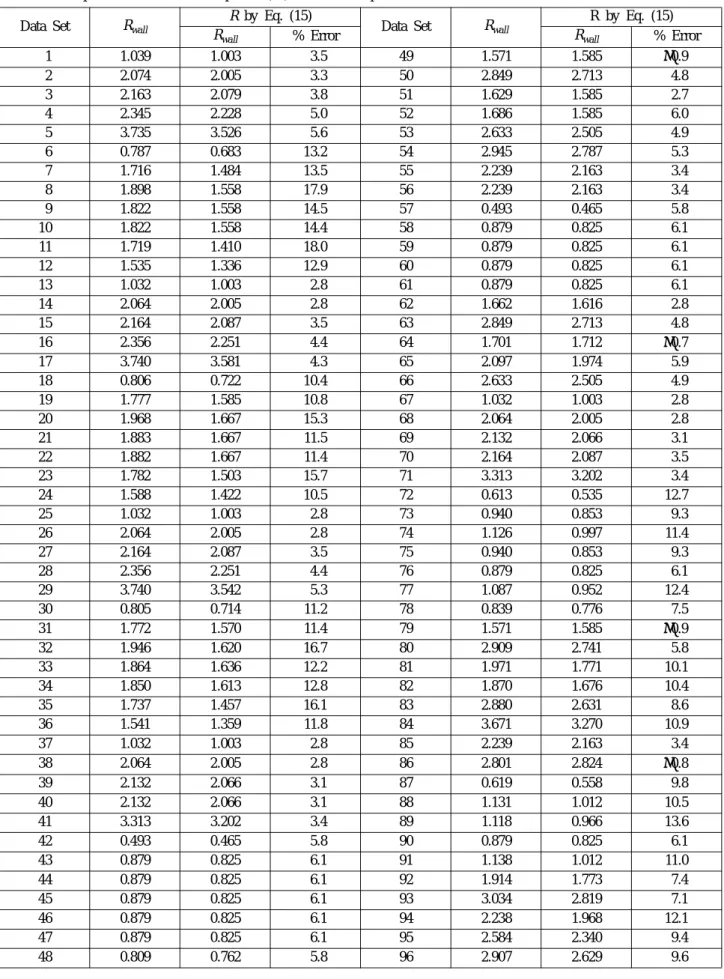
R-values generated by this program were compared with the R-values calculated using the simplified equation (15).

The results were shown in Table 2. The errors in the R- values between the computer model and the simplified model were less than 20%, which means that the simplified model successfully predicts the system R-value. Except for four cases, however, the percentage errors, which were cal- culated by (R-value by computer program-R-value by sim- plified model) / (R-value by computer program) × 100, showed positive numbers. This implies that the simplified model generally underestimates the R-value. This model was refined by fitting each coefficient in equation (15).

First, the coefficients for the linear part of the equation (15)

were fitted by multi-variable regression.

The coefficients for total thickness of solid wall (ths), total thickness of both-wall-foiled air space (tha1), and total thickness of one-side-foiled air space (tha2) were obtained by multi-variable linear regression. The BASIC program MVLR.BAS was constructed for the multi-vari- able linear regression. Among 96 data sets generated by computer model, 36 data sets, which contained foiled lay- ers, were selected for linear regression. Values of 0.027, 0.039 and 0.037 were obtained for the coefficients for total thickness of solid wall (ths), total thickness of both-wall- foiled air space (tha1), and total thickness of one-side- foiled air space (tha2), respectively. Then the non-linear part of the equation was fitted to data for the coefficient of the thickness of each none-foiled air space. MVNLR.BAS, a modified version of MVLR.BAS, which contained an additional loop to solve the non-linear problem, was used for regression. Out of the 96 data sets generated by com- puter model, 30 data sets, which constructed only with none foiled walls, were used for the regression. For non- linear part of the equation (22), 0.217 and 5.918 were obtained for the coefficients of numerator and denominator, respectively. With these results, equation (23) could be written as follows:

R_wall= 0.027ths + 0.039tha1 + 0.037tha2

+ (16)

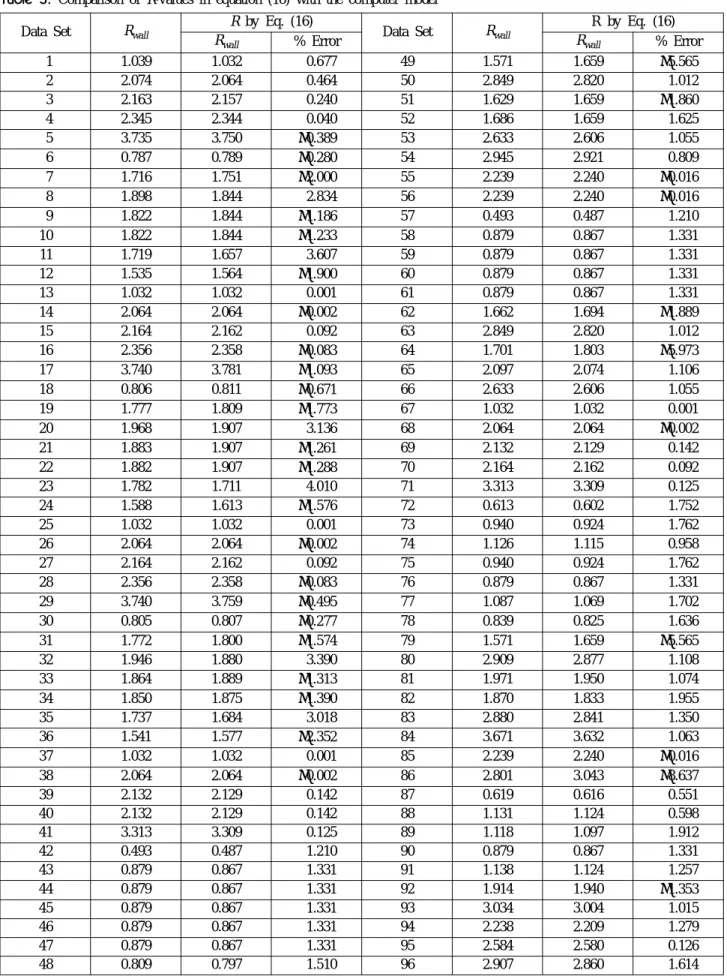
For the verification of the model, the R-values generated by computer model (See Table 2) were again compared with the R-values calculated by equation (16). As shown in Table 3, the percentage error in R-value was within 10%.

Furthermore, the percentage errors were distributed pos- itive and negative numbers, which implies that the refined model significantly improved the accuracy of the simu- lation.

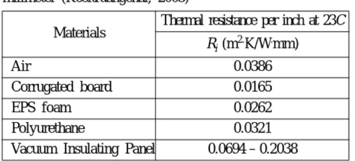
The major drawback of this equation is that thermal resis- tance generated by the solid layer cannot be differentiated between each solid material. Thus, thermal resistances per inch of each solid materials, which is summarized in Table 4, were added to the equation (16) to yield

R_wall=

+ (17)

where R_i is the thermal resistance per milimeter for the solid material of the i th layer and ths_i is the thickness of solid material of i th layer. A short table of conduction heat transfer coefficients for common insulating materials used in packaging is shown in Table 4.

0.192dair3_i 5.537+dair3_i ---

i=1

∑

0.217dair3_i 5.918+dair3_i ---

i=1

∑

R_iths_i+0.039tha1+0.037tha2

i=1

∑

0.217dair3_i 5.198+dair3_i ---

i=1

∑

Table 2. Comparison of R-values in equation (15) with the computer model Data Set R_wall R by Eq. (15)

Data Set R_wall R by Eq. (15)

R_wall % Error R_wall % Error

1 1.039 1.003 3.5 49 1.571 1.585 −0.9

2 2.074 2.005 3.3 50 2.849 2.713 4.8

3 2.163 2.079 3.8 51 1.629 1.585 2.7

4 2.345 2.228 5.0 52 1.686 1.585 6.0

5 3.735 3.526 5.6 53 2.633 2.505 4.9

6 0.787 0.683 13.2 54 2.945 2.787 5.3

7 1.716 1.484 13.5 55 2.239 2.163 3.4

8 1.898 1.558 17.9 56 2.239 2.163 3.4

9 1.822 1.558 14.5 57 0.493 0.465 5.8

10 1.822 1.558 14.4 58 0.879 0.825 6.1

11 1.719 1.410 18.0 59 0.879 0.825 6.1

12 1.535 1.336 12.9 60 0.879 0.825 6.1

13 1.032 1.003 2.8 61 0.879 0.825 6.1

14 2.064 2.005 2.8 62 1.662 1.616 2.8

15 2.164 2.087 3.5 63 2.849 2.713 4.8

16 2.356 2.251 4.4 64 1.701 1.712 −^0.7

17 3.740 3.581 4.3 65 2.097 1.974 5.9

18 0.806 0.722 10.4 66 2.633 2.505 4.9

19 1.777 1.585 10.8 67 1.032 1.003 2.8

20 1.968 1.667 15.3 68 2.064 2.005 2.8

21 1.883 1.667 11.5 69 2.132 2.066 3.1

22 1.882 1.667 11.4 70 2.164 2.087 3.5

23 1.782 1.503 15.7 71 3.313 3.202 3.4

24 1.588 1.422 10.5 72 0.613 0.535 12.7

25 1.032 1.003 2.8 73 0.940 0.853 9.3

26 2.064 2.005 2.8 74 1.126 0.997 11.4

27 2.164 2.087 3.5 75 0.940 0.853 9.3

28 2.356 2.251 4.4 76 0.879 0.825 6.1

29 3.740 3.542 5.3 77 1.087 0.952 12.4

30 0.805 0.714 11.2 78 0.839 0.776 7.5

31 1.772 1.570 11.4 79 1.571 1.585 −^0.9

32 1.946 1.620 16.7 80 2.909 2.741 5.8

33 1.864 1.636 12.2 81 1.971 1.771 10.1

34 1.850 1.613 12.8 82 1.870 1.676 10.4

35 1.737 1.457 16.1 83 2.880 2.631 8.6

36 1.541 1.359 11.8 84 3.671 3.270 10.9

37 1.032 1.003 2.8 85 2.239 2.163 3.4

38 2.064 2.005 2.8 86 2.801 2.824 −0.8

39 2.132 2.066 3.1 87 0.619 0.558 9.8

40 2.132 2.066 3.1 88 1.131 1.012 10.5

41 3.313 3.202 3.4 89 1.118 0.966 13.6

42 0.493 0.465 5.8 90 0.879 0.825 6.1

43 0.879 0.825 6.1 91 1.138 1.012 11.0

44 0.879 0.825 6.1 92 1.914 1.773 7.4

45 0.879 0.825 6.1 93 3.034 2.819 7.1

46 0.879 0.825 6.1 94 2.238 1.968 12.1

47 0.879 0.825 6.1 95 2.584 2.340 9.4

48 0.809 0.762 5.8 96 2.907 2.629 9.6

Table 3. Comparison of R-values in equation (16) with the computer model Data Set R_wall R by Eq. (16)

Data Set R_wall R by Eq. (16)

R_wall % Error R_wall % Error

1 1.039 1.032 0.677 49 1.571 1.659 −5.565

2 2.074 2.064 0.464 50 2.849 2.820 1.012

3 2.163 2.157 0.240 51 1.629 1.659 −^1.860

4 2.345 2.344 0.040 52 1.686 1.659 1.625

5 3.735 3.750 −^{0.389 53} 2.633 2.606 1.055 6 0.787 0.789 −0.280 54 2.945 2.921 0.809 7 1.716 1.751 −^{2.000 55} 2.239 2.240 −^0.016 8 1.898 1.844 2.834 56 2.239 2.240 −0.016 9 1.822 1.844 −^{1.186 57} 0.493 0.487 1.210 10 1.822 1.844 −1.233 58 0.879 0.867 1.331

11 1.719 1.657 3.607 59 0.879 0.867 1.331

12 1.535 1.564 −^{1.900 60} 0.879 0.867 1.331

13 1.032 1.032 0.001 61 0.879 0.867 1.331

14 2.064 2.064 −^{0.002 62} 1.662 1.694 −^1.889

15 2.164 2.162 0.092 63 2.849 2.820 1.012

16 2.356 2.358 −^{0.083 64} 1.701 1.803 −^5.973 17 3.740 3.781 −^{1.093 65} 2.097 2.074 1.106 18 0.806 0.811 −0.671 66 2.633 2.606 1.055 19 1.777 1.809 −^{1.773 67} 1.032 1.032 0.001 20 1.968 1.907 3.136 68 2.064 2.064 −^0.002 21 1.883 1.907 −^{1.261 69} 2.132 2.129 0.142 22 1.882 1.907 −^{1.288 70} 2.164 2.162 0.092

23 1.782 1.711 4.010 71 3.313 3.309 0.125

24 1.588 1.613 −1.576 72 0.613 0.602 1.752

25 1.032 1.032 0.001 73 0.940 0.924 1.762

26 2.064 2.064 −^{0.002 74} 1.126 1.115 0.958

27 2.164 2.162 0.092 75 0.940 0.924 1.762

28 2.356 2.358 −^{0.083 76} 0.879 0.867 1.331 29 3.740 3.759 −0.495 77 1.087 1.069 1.702 30 0.805 0.807 −^{0.277 78} 0.839 0.825 1.636 31 1.772 1.800 −1.574 79 1.571 1.659 −5.565

32 1.946 1.880 3.390 80 2.909 2.877 1.108

33 1.864 1.889 −^{1.313 81} 1.971 1.950 1.074 34 1.850 1.875 −^{1.390 82} 1.870 1.833 1.955

35 1.737 1.684 3.018 83 2.880 2.841 1.350

36 1.541 1.577 −2.352 84 3.671 3.632 1.063 37 1.032 1.032 0.001 85 2.239 2.240 −^0.016 38 2.064 2.064 −0.002 86 2.801 3.043 −8.637

39 2.132 2.129 0.142 87 0.619 0.616 0.551

40 2.132 2.129 0.142 88 1.131 1.124 0.598

41 3.313 3.309 0.125 89 1.118 1.097 1.912

42 0.493 0.487 1.210 90 0.879 0.867 1.331

43 0.879 0.867 1.331 91 1.138 1.124 1.257

44 0.879 0.867 1.331 92 1.914 1.940 −^1.353

45 0.879 0.867 1.331 93 3.034 3.004 1.015

46 0.879 0.867 1.331 94 2.238 2.209 1.279

47 0.879 0.867 1.331 95 2.584 2.580 0.126

48 0.809 0.797 1.510 96 2.907 2.860 1.614

Conclusion

One-dimensional heat transfer through the multi-layered insulating packaged were investigated using mathematical models. From Grashof number calculation, it was con- firmed that the heat transfer in the air space thinner than 13 mm was dominated by conduction rather than convection.

The heat transfer in the air space between the layers was also substantially affected by radiation. The emissivities of the surfaces were very important to characterize the radi- ation through the air space between the surfaces. If either side of the surface has a low emissivity (one or both sur- face foiled), thermal resistance of the air space increased dramatically. Otherwise, the air space between the layer provided a low thermal resistance. These factors should be considered to design the multi-layered wall structure. All of these factors were reflected in the equation (17). Using equation (17), one can effectively design the multi-layered structure for the insulating package.

Equation(17) assumed the heat transfer through the insu- lating package as one-dimensional phenomenon. As men- tioned in introduction, more factors involve in the heat transfer through the real insulating package: the three dimensional geometry of the insulating package, the geom-

etry of the product itself, the contact between the product and the insulating package, etc. These factors should be considered to explain the heat transfer through the entire insulating package.

However, this study provided the solution for the thermal resistance of the complex wall structure. In other words, the result of this study can be combined with other factors to generate the comprehensive model to predict the per- formance of the insulating package. In fact, equation (17) were applied to the model which considered all other fac- tors of the entire insulating package and resultedin a good prediction (4).

REFERENCES

1. ASHRAE. (1993). ASHRAE Handbook. Fundamentals.

Atlanta, GA: American Society of Heating, Refrigerating and Air-Conditioning Engineers.

2. Burgess, G. (1999). Practical Thermal Resistance and Ice Requirement Calculations for Insulating Packages. Packaging Technology and Science:12, 75-80.

3. Choi, S.-J. (2004). Mathematical Models to Predict the Performance of InsulatingPackages and Their Practical Uses. PH. D. Dissertation. East Lansing, MI:Michigan State University

4. Holman, J. P. (1986). Heat Transfer, 6th ed. New York, NY:

McGraw-Hill.

5. Jacob, M. (1949). Heat Transfer. New York, NY: John Wiley and Sons.

6. Kreith, F. (1973). Principles of Heat Transfer, 3rd ed. New York, NY: Intext Press.

7. Kositruangchai, N. (2003). Theoretical, Experimental and Computer Model for Package R-value Using Regular Ice and Dry Ice. Masters Thesis. East Lansing, MI: Michigan State University.

8. Stavish, L. J. (1984). Designing Insulated Packaging for Perishable in vivo Diagnostics. Medical Device and Diagnostic Industry: 6 (18), 105-108.

Table 4.Thermal resistance of various insulation materials per milimeter (Kositruangchai, 2003)

Materials Thermal resistance per inch at 23C R_i (m^2.K/W^.mm)

Air 0.0386

Corrugated board 0.0165

EPS foam 0.0262

Polyurethane 0.0321 Vacuum Insulating Panel 0.0694 – 0.2038