- - Optimizing the reconstruction filter in cone-beam CT to improve periodontal ligament space visualization: An in vitro study

(1)

https://doi.org/10.5624/isd.2017.47.3.199

Introduction

Radiographic examination of the alveolar bone is an essential step in the diagnosis of dental diseases such as periodontitis, endodontic lesions, and dental ankylosis.^1-3 In particular, assessments of the alveolar bone height, the thickness of cortical and cancellous bone, and the perio-

dontal ligament space are key for diagnosing these diseases. The periodontal ligament space is an important indica- tor of the presence of a healthy and functional periodontal ligament, as well as the relationship between the tooth root and alveolar bone. Conventional intraoral radiography is adequate for determining the width of the interproximal periodontal ligament space and bony defects,^4,5 but has some limitations in the depiction of buccolingual structures.^6-9

Recently, cone-beam computed tomography(CBCT) has been favored for periodontal evaluation because of its capability of 3-dimensional analysis.^10-12 Three-dimen-

Optimizing the reconstruction filter in cone-beam CT to improve periodontal ligament space visualization: An in vitro study

Yuuki Houno¹, Toshimitsu Hishikawa^2,*, Ken-ichi Gotoh³, Munetaka Naitoh⁴, Akio Mitani², Toshihide Noguchi², Eiichiro Ariji⁴, Yoshie Kodera¹

1Graduate School of Medicine, Nagoya University, Japan

2Department of Periodontology, School of Dentistry, Aichi Gakuin University, Japan

3Division of Radiology, Dental Hospital, Aichi Gakuin University, Japan

4Department of Oral and Maxillofacial Radiology, School of Dentistry, Aichi Gakuin University, Japan

ABSTRACT

Purpose: Evaluation of alveolar bone is important in the diagnosis of dental diseases. The periodontal ligament space is difficult to clearly depict in cone-beam computed tomography images because the reconstruction filter conditions during image processing cause image blurring, resulting in decreased spatial resolution. We examined different reconstruction filters to assess their ability to improve spatial resolution and allow for a clearer visual

ization of the periodontal ligament space.

Materials and Methods: Cone-beam computed tomography projections of 2 skull phantoms were reconstructed using 6 reconstruction conditions and then compared using the Thurstone paired comparison method. Physical evaluations, including the modulation transfer function and the Wiener spectrum, as well as an assessment of space visibility, were undertaken using experimental phantoms.

Results: Image reconstruction using a modified SheppLogan filter resulted in better sensory, physical, and quanti

tative evaluations. The reconstruction conditions substantially improved the spatial resolution and visualization of the periodontal ligament space. The difference in sensitivity was obtained by altering the reconstruction filter.

Conclusion: Modifying the characteristics of a reconstruction filter can generate significant improvement in assess

ments of the periodontal ligament space. A highfrequency enhancement filter improves the visualization of thin structures and will be useful when accurate assessment of the periodontal ligament space is necessary.(Imaging Sci Dent 2017; 47: 199-207)

KEY WORDS: Cone-Beam Computed Tomography; Image Processing, Computer-Assisted; Phantoms, Imaging;

Periodontal Ligament

This is an Open Access article distributed under the terms of the Creative Commons Attribution NonCommercial License(http://creativecommons.org/licenses/by-nc/3.0) which permits unrestricted non-commercial use, distribution, and reproduction in any medium, provided the original work is properly cited.

Imaging Science in Dentistry·pISSN 22337822 eISSN 22337830 Received March 22, 2017; Revised May 21, 2017; Accepted June 7, 2017

*Correspondence to : Dr. Toshimitsu Hishikawa

Department of Periodontology, School of Dentistry, Aichi Gakuin University, 211 Suemoridori, Chikusaku, Nagoya 4648651, Japan

Tel) 81527592150, Fax) 81527592150, Email) to[email protected]

(2)

sional reconstruction of alveolar bone offers a precise diagnosis of furcation and intraosseous defects in order to plan periodontal surgery and regenerative therapy. CBCT also allows observation of the tooth root morphology;

however, the root boundary is difficult to set definitively because CBCT images have no threshold to define the root dentin. Furthermore, image blurring can result from the partial volume effect and artifacts sometimes obscure the gray value of the boundary. To our knowledge, there have been no studies investigating the successful depiction of tooth root morphology in CBCT images. Clear discrimination of the periodontal ligament space could as- sist in visualizing the tooth root morphology.

The healthy periodontal ligament space is approximately 0.2mm thick, and the spatial resolution of CBCT is sometimes insufficient to depict this space.^13-15 The spatial resolution of CBCT images is determined by many factors, including tube current, hardware specifications, and image reconstruction software. Although hardware specifications impose some fixed limitations,¹⁶ image reconstruction algorithms provide some flexibility. In recent years, research on several reconstruction algorithms of multi-slice computed tomography(CT) scans, such as it- erative reconstruction, have been developed;¹⁷ however, the conventional filtered back-projection(FBP) method and the Feldkamp algorithm-one of the most widely referenced algorithms¹⁸-are still popular approxima- tions for dental CBCT reconstruction. Therefore, we have focused on the image reconstruction filter in the FBP algorithm to attempt to reduce image blur and improve spatial resolution.¹⁹ One key method to improve the results of CT imaging is changing the reconstruction filter to optimize image characteristics that depend on the region of interest. For example, in chest CT imaging, a reconstruction filter that emphasizes the high-frequency component has been applied,²⁰ and in soft-tissue CT imaging, a reconstruction filter that suppresses the high-frequency component has been used. However, in dental CBCT applications, reconstruction filters are rarely available to alternate and improve image quality directly for diagnostic purposes, such as discerning a narrow space between structures with high CT values.

In this study, we examined various reconstruction filters in the FBP algorithm to evaluate the periodontal ligament space of a dry skull phantom as a sample of a narrow structure and to verify that the rendering of the fine, hard-tissue structures can be improved. We also evaluated the filters’ physical and quantitative effects with the use of an experimental phantom.

Materials and Methods

Image acquisition and reconstruction

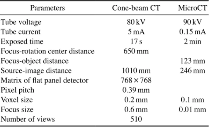
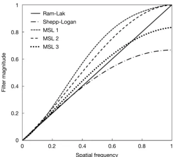
In this study, a dental CBCT scanner(Alphard-3030, Asahi Roentgen Industry Co. Ltd, Kyoto, Japan) was employed. Images were acquired from 4 different areas in 2 skull phantoms(Kyoto Kagaku Co. Ltd, Kyoto, Ja- pan), a wire phantom, a water phantom, and an artificial periodontal ligament phantom. The CBCT exposure conditions are shown in Table 1. The CBCT scanner can ac- quire both raw projection data and reconstructed 2-dimensional axial images(the Alphard’s default images). The default images from the Alphard device were reconstructed with its default application using a SheppLogan filter and additional confidential image processing. The raw projection data were reconstructed into modified axial images using 5 filters with a software package called Open Source Conebeam Reconstructor(OSCaR).²¹ OSCaR is written in Matlab code(MathWorks Co. Ltd, Natick, MA, USA) and uses the FBP method and the Feldkamp algorithm. Two well-known filters(RamLak and SheppLo- gan) were employed as references, and 3 filters were de- signed to increase the high-frequency component based on the SheppLogan function(Fig. 1).^22,23 The formulae of the filters were as follows:

Modified SheppLogan(MSL) 1:

2 2 2 Skull phantoms used for visual evaluations

CBCT data from 2 commercially available skull phan-

Table 1. Cone-beam CT and microCT exposure conditions

Parameters Cone-beam CT MicroCT

Tube voltage Tube current Exposed time

Focusrotation center distance Focusobject distance Sourceimage distance Matrix of flat panel detector Pixel pitch

Voxel size Focus size Number of views

80kV 5mA 17s 650mm 1010mm 768×768 0.39mm

0.2mm 0.6mm 510

90kV 0.15mA

2min 123mm 246mm

0.1mm 0.01mm

(3)

toms made with actual human dry skulls(age and sex unknown) embedded in soft tissue-equivalent resin were used for visual evaluation of periodontal ligament space visibility. The acquired image regions from the 2 skull phantoms included the maxillary anterior region and mandibular anterior region of 1 phantom and the mandibular anterior region and mandibular molar region of the other phantom.

The OSCaR reconstructed images and the default images of the skull phantoms were compared using the Thur- stone method of paired comparison,²⁴ and a scale value was calculated. Six image sets were compared using a round-robin formula for 4 different jaw regions. Image clarity of the periodontal ligament space boundaries was evaluated by 3 periodontists and 3 radiologists with >5 years of clinical experience. In total, 60 comparisons were performed by each observer. All observations were performed randomly on a 20.1-inch medical monitor(Radi- Force G20, EIZO Co. Ltd, Hakusan, Japan) operating at a resolution of 1200×1600 pixels. Before the viewing ses- sions, examiners were calibrated with test images and the evaluation point was explained. Examiners were allowed to change the window width/level and slice positions using ImageJ 1.47b software(a Java-based image processing program) and a Digital Imaging and Communications in Medicine viewer, both developed at the National Insti- tutes of Health(MD, USA). Slice positions of the 2 obser-

vation images were synchronized, and an observational time limit was not specified. This observation study was approved by the Nagoya University ethics board(approval number 12-322).

The paired comparisons were statistically evaluated by analysis of variance using the F test(α<.05) and the yardstick method.²⁵

Physical evaluation

To confirm image characteristics, the modulation transfer function(MTF) and Wiener spectrum(WS) were calculated.²⁶ The MTF, which is calculated from the point spread function, is the established method for characteriz- ing the spatial response of an image. In this study, a wire method was employed for the MTF calculation,²⁷ using a wire phantom made of copper wire(0.28mm in diameter) and a water-filled cylindrical acrylic container(150mm in diameter). The WS is a valuable tool for assessing the noise power of an image in the spatial frequency domain and was calculated by the virtual slit method,^28,29 using a cylindrical water phantom made only of a water-filled cylindrical acrylic container. Both calculations were performed using ImageJ visualization and measurement software and Excel 2010(Microsoft Co., Ltd., Redmond, WA, USA). We assessed images using the default reconstruction of the Alphard apparatus and reconstruction with the filter that was rated highest for visual evaluation.

To distinguish the measurable periodontal ligament space widths as a parameter for periodontal ligament space visibility, we used the periodontal ligament phantom to compare the gray values between the alveolar bone equivalent and the simulated periodontal ligament space.

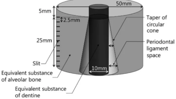
The periodontal ligament phantom was made from 2 different materials: an alveolar bone-equivalent substance and a dentin-equivalent substance produced as a solid column by Kyoto Kagaku Co. Ltd(Kyoto, Japan). The CT values of each block, confirmed by whole-body CT (Asteion Super 4 TSX021B, Toshiba Medical Systems Co. Ltd, Otawara, Japan), were 272 and 1893, respec- tively. These blocks were shaped into a center post with a fixed circumference by Tokai Giken Co. Ltd(Ena, Japan) and then assembled to simulate a periodontal ligament space. The dimensional tolerance of the cutting work was estimated to be <0.02mm. The composition of the materials and the final shape are shown in Figure 2. Tapering of a circular cone-shaped hole bored in the center of the circumference simulated changes in the width of the periodontal ligament space in the range of 0.0-1.0mm. The periodontal ligament phantom was placed in water, and

Fig. 1. Reconstruction filters prepared for observation of the periodontal ligament space. Modified SheppLogan(MSL) 1 shows the most highly enhanced highfrequency component, MSL 2 shows medium enhancement, and MSL 3 shows the leastenhanced high-frequency component.

1

0.8

0.6

0.4

0.2

0

Ram-Lak Shepp-Logan MSL 1 MSL 2 MSL 3

0 0.2 0.4 0.6 0.8 1 Spatial frequency

Filter magnitude

(4)

the periodontal ligament space filled with water to simulate biological conditions.

Axial images of the periodontal ligament phantom were obtained by CBCT(the default reconstruction and reconstruction with the highest rated filter) and microscopic CT(micro-CT high-resolution(R_mCT2, Rigaku Co. Ltd, Tokyo, Japan) as a reference. The microCT machine has microfocus Xray tubes and a highresolution flatpanel detector. The gantry is 194mm in diameter, and the maximum field of view is 73×57mm. The voxel size and the field of view were set to 0.1mm³ and 48×48mm, respec- tively. The phantom coordinate axes were adjusted to match those of the CBCT as much as possible. Exposure conditions using the microCT scanner are shown in Table 1. The acquired images of each modality were converted to gray values for each pixel, and the gray values of the periodontal ligament space and the alveolar bone were extracted using Excel 2010. To measure the periodontal ligament space, we compared the gray values of the periodontal ligament space and the alveolar bone in a total of 10 slices representing a 0.1-mm change in the periodontal ligament space. For the statistical treatment of the gray values, the lower threshold level showing the presence of bone was set at the lower limit of the 95% CI of alveolar bone. The 95% CI was approximately the same as the mean value±2 standard deviations(SDs). Thus, if the value obtained by subtracting the gray value of the estimated region of the periodontal ligament space from the mean value±2 SD of the alveolar bone was positive, it was considered to be a significant difference and confirmed the existence of a periodontal ligament space.

To visualize the effect of gray-value alteration by the reconstruction filter, the gray-value profiles of the periodontal ligament space were compared using polar-transformed images generated in ImageJ. The polar images

were stacked at an angle to avoid any noise influence.

Results

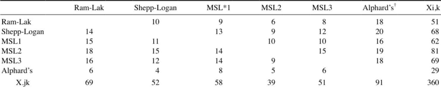
The representative images obtained from the skull phantoms are shown in Figure 3. The default images obtained using the Alphard apparatus were smooth, but the reconstructed images using the MSL function were rough in appearance. The raw choice matrix is shown in Table 2.

The results of the Thurstone paired comparison using these images are shown in Figure 4. The resulting scale values were calculated as follows: default image: 0, Ram- Lak: 43, MSL 1: 64, SheppLogan: 76, MSL 3: 77, MSL 2: 100. The image that best distinguished the periodontal ligament space was the one reconstructed with MSL 2.

The default images used in clinical settings yielded the worst result. The yardstick method revealed a significant difference between each filter, with differences in scale values ≥28. Thus, visibility of the periodontal ligament space was significantly poorer in the MSL 1, RamLak, and Alphard default images than in the MSL 2 images.

The MTF and WS values were compared, using water and wire phantoms, to verify the changes in image characteristics between MSL 2 and Alphard default images.

The values for MTF and WS are shown in Figure 5. The MTF values reveal that the spatial resolution in the MSL 2 images was higher than that in the default images. The WS values increased when using a reconstruction filter that emphasized highfrequency components; MSL 2 images had particularly high WS values up to the highfrequency domain, which indicates greater granularity.

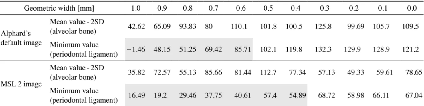
To confirm the minimum discriminable width, axial images of the periodontal ligament phantom reconstructed with 2 conditions were compared using the periodontal ligament phantom. The subtracted gray values of each condition are shown in Table 3. The gray cells represent- ed the minimum values smaller than 2 SDs, and these cells were presumed to be the periodontal ligament space.

A positive value indicated that the gray value of the periodontal ligament space was lower than the value of the mean -2 SDs of alveolar bone, and the periodontal ligament space was determined. A negative value indicated that the space could not be distinguished, because the periodontal ligament space was assimilated into the bone.

Simulated periodontal ligament spaces thinner than 0.3 mm could not be observed under either condition. The discriminating width limits were 0.6mm for the Alphard default images and 0.4mm for the MSL 2 images.

The gray value profiles of the simulated periodontal

Fig. 2. Diagram of the periodontal ligament phantom.

(5)

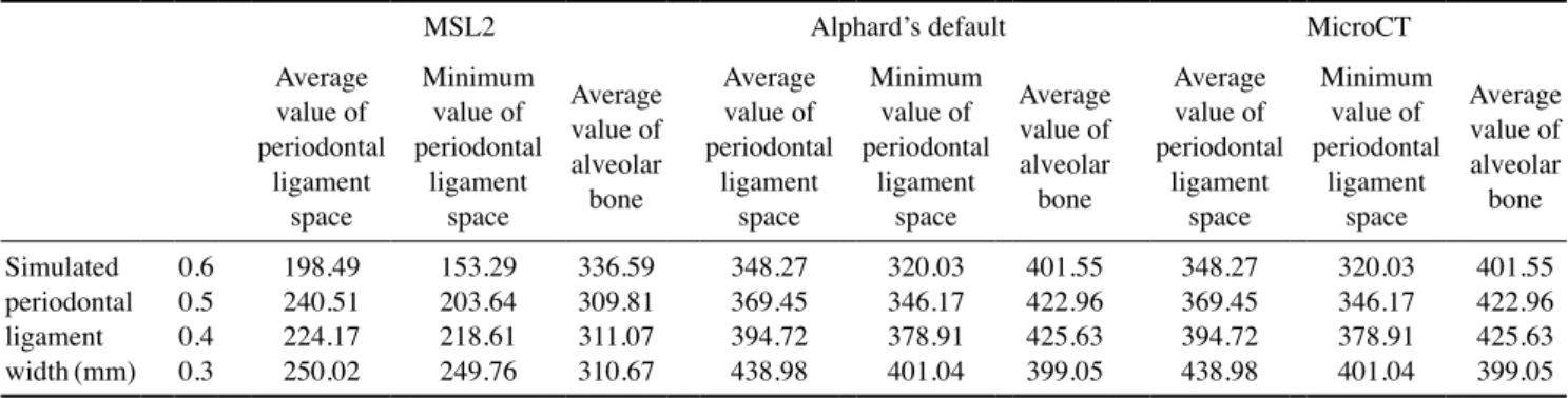
ligament space are shown in Figure 6. The representative value of the simulated periodontal ligament space in the polartransformed images is shown in Table 4. The MSL

2 profile represents a sharp decrease and a clear apex of gray values at the simulated space widths of 0.5 and 0.4 mm but not at the 0.3-mm profile. The Alphard default

Table 2. An aggregate raw choice matrix for 6 respondents

RamLak SheppLogan MSL*1 MSL2 MSL3 Alphard’s^† Xi,k

RamLak SheppLogan MSL1MSL2 MSL3Alphard’s

1415 1816 6

10 1115 12 4

913

1414 8

6 9 10 9 5

812 1015

6

1820 1619 18

51 68 62 81 69 29

X.jk 69 52 58 39 51 91 360

*MSL: modified SheppLogan, ^†Alphard’s: Alphard’s default image

Fig. 3. Typical default images from the Alphard apparatus, and images reconstructed by each filter. A: Default, B: RamLak, C: Shepp

Logan, D: modified SheppLogan(MSL) 1, E: MSL 2, F: MSL 3.

A B C

D E F

Fig. 4. The scale value calculated by the Thurstone pairedcomparison method. A disparity in the scale value larger than 28 was considered a significant difference.

(6)

image profile showed a gentle degradation of gray values for each width. As a reference, the microCT profile demonstrated steady degradation of gray-value differences in relation to the reduction in size of the periodontal ligament space. The appearance of the profiles graphi- cally explains the results of the statistical analysis with a 95% CI.

Discussion

In this study, the optimal reconstruction filter was MSL 2, which had a high-frequency component enhancement.

The results of the paired comparisons revealed that the images enabled the observer to clearly view the boundary of the periodontal ligament space. The MTF and WS results confirmed that MSL 2 reconstruction improved image sharpness despite increased noise. These physical

evaluations suggest that sharp images enhance the visualization of the periodontal ligament space; in other words, the visibility of the periodontal ligament space is not markedly affected by noise. Therefore, the images used for visual assessment by the observers were provided as a stack instead of a single slice. The observers recognized the continuous structure by comparing the plurality of slices and then provided a visual evaluation of the periodontal ligament space. The visual evaluation may have been less influenced by image noise in the setting of this study. The images for visualization of periodontal bone may use high-frequency enhancement. Therefore, our data comprise the essential components for precise visualization of periodontal hard-tissue structures.

The highest spatial resolution of the CBCT apparatus employed in this study was a square voxel of 0.1mm. In the imaging mode with 0.1-mm³ resolution, the image

Fig. 5. The modulation transfer function(MTF) and Wiener spectrum(WS) of a modified SheppLogan(MSL) 2 image and the default image obtained using the Alphard apparatus.

1.2

1

0.8

0.6

0.4

0.2

0

10000

1000

100

10

1

0.1

MSL 2 MSL 2

Alphard's default

0 0.5 1 1.5 2 2.5 Spatial frequency[cycles/mm]

0 0.5 1 1.5 2 2.5 3 Spatial frequency[cycles/mm]

MTF WS value[mm2 ]

Table 3. Discriminable width of the simulated periodontal ligament space in the periodontal ligament phantom

Geometric width [mm] 1.0 0.9 0.8 0.7 0.6 0.5 0.4 0.3 0.2 0.1 0.0

Alphard’s default image

Mean value-2SD

(alveolar bone) 42.62 65.09 93.83 80 110.1 101.8 100.5 125.8 99.69 105.7 109.5 Minimum value

(periodontal ligament) -1.46 48.15 51.25 69.42 85.71 102.1 119.8 132.3 129.9 128.9 121.2

MSL 2 image

Mean value-2SD

(alveolar bone) 35.82 72.57 55.13 85.66 81.44 112.7 77.34 57.13 49.33 59.61 78.65 Minimum value

(periodontal ligament) 16.49 19.2 29.46 37.75 40.61 57.4 54.89 68.72 58.98 66.11 67.04

(7)

reconstruction is performed using data mainly obtained from a decentralized area of the Xray beam. However, we conducted the experiments in the imaging mode using the central area of the Xray beam, although the spatial resolution was inferior. The spatial resolution could be considered insufficient for depicting the thickness of the periodontal ligament space; however, it is noteworthy that changing the reconstruction filter increased the spatial resolution under conditions that are generally applicable to many currently available devices.

This study successfully evaluated differences between images, even though the filtering effect was predicted to yield relatively small differences in CBCT images. Using the Thurstone paired-comparison method, which is effect- ive in distinguishing similar subjects, we clearly distinguished differences between the reconstructed images and succeeded in scaling all the filters. The comparison of MSL 1 and MSL 2 shows that the enhancement of the high-frequency component had a maximum value, above

which image degradation occurs. This degradation ap- pears to be caused by 2 main factors: hard-tissue artifacts and noise enhancement by high-frequency enhancement.

These results of the sensory and physical evaluations car- ried out in this study correspond well with the results of a previous study.¹⁹

In a quantitative assessment, the normal periodontal ligament width is difficult to depict with conventionally reconstructed CBCT images, partly because the space that exists between similar pixel values is difficult to visualize.³⁰ The default CBCT images resulted in the detection of a 0.4-0.6-mm interval; this was inferior to the results of a previous study.^14,15 This is partly because the periodontal ligament phantom replicated the nonuniform morphology of the periodontal ligament space, and the space was filled with water. Given the gradually changing width of the periodontal ligament space and the relatively large voxel size, it is likely that the partial volume effect influenced our results. Additionally, the periodontal ligament

Fig. 6. Grayvalue profiles of the simulated periodontal ligament space obtained by polar transformation.

1600 1400 1200 1000 800 600 400 200 0

3000 2500 2000 1500 1000 500 0 -500 0.6

0.50.4 0.3

Modified Shepp Logan 2 Alphard's default image microCT

0 5 10 15 20 25 Position

Relative pixel value Relative pixel value Relative pixel value

Table 4. The representative gray-values of the simulated periodontal ligament space in the polar transformed image

MSL2 Alphard’s default MicroCT

Average value of periodontal

ligament space

Minimum value of periodontal

ligament space

Average value of alveolar

bone

ligament space

Average value of alveolar

bone

ligament space

Average value of alveolar bone Simulated

periodontal ligament width(mm)

0.60.5 0.40.3

198.49 240.51 224.17 250.02

153.29 203.64 218.61 249.76

336.59 309.81 311.07 310.67

348.27 369.45 394.72 438.98

320.03 346.17 378.91 401.04

401.55 422.96 425.63 399.05

348.27 369.45 394.72 438.98

320.03 346.17 378.91 401.04

401.55 422.96 425.63 399.05

*MSL: modified SheppLogan

(8)

space was filled with water to mimic biological conditions; this was not the case in previous studies. Thus, our results, although inferior, may be closer to what may be achieved with living patients.

MSL 2 improves the resolution of dental CBCT with- out having to replace current hardware. This means that image quality can be improved with little associated ex- pense or any increase in radiation dose-it only requires a software update. However, although sharp images were obtained by image processing, they were not sufficient to depict the periodontal ligament. To obtain sharper images, a highresolution detector and an Xray tube with a small focus are considered to be essential, but the exposure conditions eventually lead to an increase in the radiation dose.¹⁹ Because the right balance of noise and sharpness is required, a suitable reconstruction filter is useful in the dental field.

In conclusion, we determined that a high-frequency enhancement filter improved spatial resolution and allowed for better measurement of the periodontal ligament space.

We also confirmed that using an image with a high-frequency component improved the evaluation of a periodontal ligament phantom. However, higher spatial resolution led to increased noise levels. This study was successful in finding a suitable reconstruction filter to discern the periodontal ligament space. However, for clinical applications, the various characteristics of image quality should be taken into account, including measurement of the con- trast-to-noise ratio; this will require further optimization.

Thus, future investigations can verify the clinical benefits of altering the reconstruction filter by ascertaining the importance of an appropriate compromise between sharpness and smoothing in order to achieve improved diagnostic accuracy or to save time. Apart from periodontal diagnosis, we believe that our method has the potential to improve periodontal treatment by using 3-dimensional visualization and stereolithography technology, espe- cially in regenerative therapy when a scaffold material is applied. The development of clear and precise imaging techniques will improve such applications as part of periodontal treatment.

Acknowledgements

Our heartfelt appreciation goes to Dr. Kazuhito Yoshi- da, Dr. Hidehiko Kamei, Dr. Miwa Nakayama, and Dr.

Shinsuke Sugiura for their contribution to the observation experiments. We would also like to express our gratitude to Mr. Hirohisa Kato and Mr. Mitsuteru Watarai for their

cooperation in the development of the periodontal ligament phantom. We also appreciate the help from Dr. Shuichiro Kobayashi with the periodontal ligament phantom image acquisition.

References

1. Corbet EF, Ho DK, Lai SM. Radiographs in periodontal dis- ease diagnosis and management. Aust Dent J 2009; 54 Suppl 1:

S2743.

2. Gröndhal HG, Huumonen S. Radiographic manifestations of periapical inflammatory lesions: how new radiological techniques may improve endodontic diagnosis and treatment plan- ning. Endod Topics 2004; 8: 5567.

3. Andersson L, Blomlöf L, Lindskog S, Feiglin B, Hammar- ström L. Tooth ankylosis. Clinical, radiographic and histologi- cal assessments. Int J Oral Surg 1984; 13: 42331.

4. de Faria Vasconcelos K, Evangelista KM, Rodrigues CD, Estrela C, de Sousa TO, Silva MA. Detection of periodontal bone loss using cone beam CT and intraoral radiography.

Dentomaxillofac Radiol 2012; 41: 649.

5. Esmaeli F, Shirmohammadi A, Faramarzie M, Abolfazli N, Rasouli H, Fallahi S. Determination of vertical interproximal bone loss topography: correlation between indirect digital radiographic measurement and clinical measurement. Iran J Radiol 2012; 9: 837.

6. Baksi BG. Measurement accuracy and perceived quality of imaging systems for the evaluation of periodontal structures.

Odontology 2008; 96: 5560.

7. Fuhrmann RA, Wehrbein H, Langen HJ, Diedrich PR. Assess

ment of the dentate alveolar process with high resolution computed tomography. Dentomaxillofac Radiol 1995; 24: 50

8. Hishikawa T, Izumi M, Naitoh M, Yoshinari N, Kawase H, 4.

Matsuoka M, et al. Effects of the vertical projection angle in intraoral radiography on the detection of furcation involve- ment of the mandibular first molar. Oral Radiol 2011; 27: 102

9. Misch KA, Yi ES, Sarment DP. Accuracy of cone beam com-7.

puted tomography for periodontal defect measurements. J Periodontol 2006; 77: 1261-6.

10. Walter C, Kaner D, Berndt DC, Weiger R, Zitzmann NU.

Three-dimensional imaging as a pre-operative tool in decision making for furcation surgery. J Clin Periodontol 2009; 36:

250-7.

11. Naitoh M, Yamada S, Noguchi T, Ariji E, Nagao J, Mori K, et al. Three-dimensional display with quantitative analysis in alveolar bone resorption using cone-beam computerized tomography for dental use: a preliminary study. Int J Periodontics Restorative Dent 2006; 26: 60712.

12. Bayat S, Talaeipour AR, Sarlati F. Detection of simulated periodontal defects using cone-beam CT and digital intraoral radiography. Dentomaxillofac Radiol 2016; 45: 20160030.

13. Nemtoi A, Czink C, Haba D, Gahleitner A. Cone beam CT: a current overview of devices. Dentomaxillofac Radiol 2013;

42: 20120443.

(9)

14. Ozmeric N, Kostioutchenko I, Hägler G, Frentzen M, Jervøe

Storm PM. Conebeam computed tomography in assessment of periodontal ligament space: in vitro study on artificial tooth model. Clin Oral Investig 2008; 12: 2339.

15. JervøeStorm PM, Hagner M, Neugebauer J, Ritter L, Zöller JE, Jepsen S, et al. Comparison of conebeam computerized tomography and intraoral radiographs for determination of the periodontal ligament in a variable phantom. Oral Surg Oral Med Oral Pathol Oral Radiol Endod 2010; 109: e95-101.

16. Bushberg JT, Seibert JA, Leidholdt EM, Boone JM. The essential physics of medical imaging. 2nd ed. Philadelphia: Lip- pincott Williams & Wilkins; 2002. p. 3689.

17. Hsieh J, Nett B, Yu Z, Sauer K, Thibault JB, Bouman CA. Re- cent advances in CT image reconstruction. Curr Radiol Rep 2013; 1: 39-51.

18. Feldkamp LA, Davis LC, Kress JW. Practical conebeam algorithm. J Opt Soc Am A 1984; 1: 6129.

19. Lee SW, Lee CL, Cho HM, Park HS, Kim DH, Choi YN, et al. Effects of reconstruction parameters on image noise and spatial resolution in cone-beam computed tomography. J Ko- rean Phys Soc 2011; 59: 282532.

20. Worthy S. High resolution computed tomography of the lungs.

BMJ 1995; 310: 615-6.

21. Rezvani N, Aruliah D, Jackson K, Moseley D, Siewerdsen J.

SUFFI16: OSCaR: an opensource conebeam CT reconstruction tool for imaging research. Med Phys 2007; 34: 2341.

22. Ramachandran GN, Lakshminarayanan AV. Threedimension- al reconstruction from radiographs and electron micrographs:

application of convolutions instead of Fourier transforms.

Proc Natl Acad Sci U S A 1971; 68: 223640.

23. Shepp LA, Logan BF. The Fourier reconstruction of a head section. IEEE Trans Nucl Sci 1974; 21: 2143.

24. Thurstone LL. A law of comparative judgment. Psychol Rev 1927; 34: 27386.

25. Scheffe H. An analysis of variance for paired comparisons. J Am Stat Assoc 2012; 47: 381400.

26. Rossmann K. Point spread-function, line spread-function, and modulation transfer function. Tools for the study of imaging systems. Radiology 1969; 93: 257-72.

27. Nickoloff EL. Measurement of the PSF for a CT scanner: appropriate wire diameter and pixel size. Phys Med Biol 1988;

33: 149-55.

28. Boedeker KL, Cooper VN, McNittGray MF. Application of the noise power spectrum in modern diagnostic MDCT: part I. Measurement of noise power spectra and noise equivalent quanta. Phys Med Biol 2007; 52: 4027-46.

29. Boedeker KL, McNittGray MF. Application of the noise power spectrum in modern diagnostic MDCT: part II. Noise power spectra and signal to noise. Phys Med Biol 2007; 52:

4047-61.

30. Barrett J, Keat N. Artifacts in CT: recognition and avoidance.

Radiographics 2004; 24: 1679-91.