Vol. 19, No. 12 pp. 14-24, 2018
General inflation and bifurcation analysis of rubber balloons
Moon Shik Park
Department of Mechanical Engineering, Hannam University
고무풍선의 일반화 팽창 및 분기 해석
박문식
한남대학교 기계공학과
Abstract Several typical hyper-elastic constitutive models that encompass both conventional and advanced ones were investigated for the application of instability problems, including the biaxial tension of a rubber patch and inflation of spherical or cylindrical balloons. The material models included the neo-Hookean model, Mooney-Rivlin model, Gent model, Arruda-Boyce model, Fung model, and Pucci-Saccomandi model. Analyses can be done using membrane equations with particular strain energy density functions. Among the typical strain energy density functions, Kearsley's bifurcation for the Treloar's patch occurs only with the Mooney-Rivlin model. The inflation equation is so generalized that a spherical balloon and tube balloons can be taken into account. From the analyses, the critical material parameters and limit points were identified for material models in terms of the non-dimensional pressure and inflation volume ratio. The bifurcation was then identified and found for each material model of a balloon. When the finite element method was used for the structural instability problems of rubber-like materials, some careful treatments required could be suggested. Overall, care must be taken not only with the analysis technique, but also in selecting constitutive models, particularly the instabilities.
요 약 몇 가지 전형적인 기존 및 진보된 초탄성 구성모델들의 고무패치 이축인장 및 구형 또는 원통형 풍선 팽창에서의 불안정성에 대해서 밝힌다. 적용할 구성모델은 neo-Hookean 모델, Mooney-Rivlin 모델, Gent 모델, Arruda-Boyce 모델, Fung 모델, Pucci-Saccomandi 모델 등이다. 팽창 및 분기 해석은 이들 변형에너지 함수들의 막 방정식을 이용하여 수행할 수 있다.
해석에는 사각패치에 대한 Kearsley의 분기현상, 고무풍선의 일반화 한 팽창현상, 고무풍선의 분기현상을 다룬다. 이들 변형 에너지 함수들 중에서도 오직 Mooney-Rivlin 모델에서만 Kearsley의 분기현상이 일어남을 확인하였다. 팽창 방정식은 구형 풍선과 원통형 풍선을 함께 다룰 수 있도록 일반화 시켰다. 팽창해석에 의하여 극한점과 임계 물성치들을 무차원 압력 및 팽창 부피의 항들로 구하였다. 그렇게 구해진 결과들로부터 분기현상을 구할 수 있었다. 또한 유한요소법을 사용하여 고무류 의 구조적 불안정 문제들을 다룰 때 필요한 특별한 조처에 대해서 제안하였다. 결론적으로 고무류의 불안정성을 포함하는 문제를 다룰 때는 해석기법은 물론 구성모델의 선택에 따라 결과가 달라질 수 있으므로 신중한 처리가 요구된다.
Keywords : rubber-like material, inflation instability, bifurcation analysis, hyper-elasticity, finite element analysis
This work was supported by a 2018 Research Grant from the Hannam University.
*Corresponding Author : Moon Shik Park(Hannam Univ.) Tel: +82-42-629-8057 email: ms.park@hannam.kr
Received August 31, 2018 Revised October 8, 2018 Accepted December 7, 2018 Published December 31, 2018
1. Introduction
Rubbery materials are well-known and diverse not only to our everyday living but to engineering and
medical use. It exhibit hyper-elasticity even when it is extended up to 5 to 15 times to the original length.
Spherical balloons from the dollar-store may show limiting chain extensibility of around 5 while typical
biological soft tissues such as human arteries can be stretched up to 2 or less[1,2]. For their higher extensibility and complicated nonlinear nature of deformation it is well known that rubber-like materials may show various kinds of instabilities including bifurcations.
Rubber balloons may also exhibit inflation instability[1,3]. Tube balloons may exhibit inflation instability as well as bifurcation[4]. Treloar's patch of particular rubber material may show in-plane bifurcation for equi-biaxial tension[5]. Compressed or bent rubber blocks may exhibit wrinkling instability on the compression surface[6]. Various inflation instabilities of rubber balloons are well documented in the literature like Kanner and Horgan[7].
Constitutive models for rubber materials are various in their mechanics and behaviors. Some material models can represent those modes of deformations while others cannot. A recent advancement of constitutive model was done by Gent and Arruda-Boyce. Gent proposed very simple phenomenological model that can represent various types of deformation[8]. Arruda and Boyce used eight molecular chain model to derive the constitutive equation[9].
This study will investigate features of representing instabilities and bifurcations of several rubber material models not only in analytic manner but also by finite element method. From time to time finite element method fails to capture unstable phenomena of rubber-like materials because of numerical instabilities.
The reason for that and some remedies will be suggested in modeling finite element analysis. Firstly the Kearsley's bifurcation in biaxially loaded rubber sheet will be presented. Secondly inflation of ball and tube balloon is analyzed by the single general inflation equation. Specific material parameter that causes inflation instabilities will be found and presented for each material model. Finally bifurcation of tube balloon is identified and analyzed either by analytic method and finite element method.
2. Theory
2.1 Basic equations
Rubber-like materials and bio-materials such as soft tissue and arterial wall can be modeled as an incompressible hyper-elastic material. For incompressible hyper-elastic continuum materials, mechanical properties are derived in terms of strain energy density function W. Letting F be the deformation gradient tensor and B=FFT be the left Cauchy-Green tensor, the strain invariants can be derived in terms of B or principal stretches λ1,λ2,λ3 as follows,
2 3 2 2 2 1 1= Btr =λ +λ +λ
I (1a)
2 1 2 3 2 3 2 2 2 2 2 1 2 2 2
2=1[(trB) −(trB )]=λλ +λλ +λλ
I (1b)
2 3 2 2 2 1 3=detB=λλλ
I (1c)
Because of the incompressibility, λ1λ2λ3=1 or 1
detF= and I3=1. The second invariant can also be expressed as 32
2 2 2 1 2
−
−
− + +
=λ λ λ
I in case of incompressible materials. Then strain energy density function can be defined by
) , (I1 I2 W
W= (2)
From the strain energy density function, constitutive equation in terms of Cauchy stress tensor σ and the left Cauchy-Green tensor B is written by
1 2
1 2
2 − −
+
−
= 1 B B
σ p W W (3)
where 1=δijeˆi⊗eˆj, W1=∂W∂I1, W2=∂W ∂I2 and p is a hydrostatic pressure due to the incompressibility constraint. And δij is the Kronecker delta and eˆ is i a unit vector in Cartesian coordinate systems. Nominal or engineering strain tensor S can be related to the Cauchy stress tensor σ by
−T
= Fσ
S (4)
In principal stretch modes, nominal stress in each direction is Sα=σαλ−α1 and Cauchy stress can be derived by
) (
2 1 2− 2 −2 +
−
= α α
α λ λ
σ p W W (5)
where α=1, 2 or 3 represent each principal direction.
Equation (5) represents membrane behavior of hyper-elastic materials and the following form of constitutive equations can be obtained.
) (
) (
2 12 22 1 23 2
2
1 σ λ λ W λ W
σ − = − + (6a)
) (
) (
2 22 23 1 21 2
3
2 σ λ λ W λ W
σ − = − + (6b)
) (
) (
2 12 23 1 22 2
3
1 σ λ λ W λ W
σ − = − + (6c)
2.2 Constitutive models
Strain energy density functions have been proposed basically in phenomenological ways or in micro-mechanical theories such as molecular network of Gaussian chains. Most simple yet representative both to experimental and theoretical basis is the following neo-Hookean model
) 3 2(1−
=G I
WnH (7)
depending on single material constant which is the infinitesimal shear modulus G and one strain variable
I . In molecular terms, a homogenized behavior of an 1
isotropic network of ideal Gaussian chains results in this model[5].
Improvement over the neo-Hookean model can be done mathematically by expanding with the second strain variable I . Mooney and Rivlin suggested the 2
following model
)]
3 )(
1 ( ) 3 (
2[ 1− + − 2−
=G I I
WMR α α (8)
where 0<α≤1 is a dimensionless material parameter.
Mooney-Rivlin model is for sure phenomenological one and one of the most popular models in modeling structures with rubber-like materials. One of the more complicated theoretical models is Arruda and Boyce's eight chain model[9] which can represent limiting chain extensibility observed when severe hardening is occurred during elongation of the specimen:
) 3
2 ( 1
5
1 2 2 k k
k k
m k
AB C I
W =
∑
−= λ −
μ
(9)
where μ and λm are material parameters relating shear modulus G with the limiting chain extensibility λm
and Ck are coefficients.
67375 ) 42039 875
513 175
99 5 1 3
( 2 4 6 8
m m
m m
G=μ + λ + λ + λ + λ
(10a)
1=1
C , 10
1
2=
C , 525 11
3=
C , C4=350019 , 336875 519
5= C
(10b)
Phenomenological model that can represent limiting chain extensibility similar to Arruda-Boyce model is the following Gent model[8].
3) 1 2 ln(
1 m m
GE J
J I
W =−G − −
(11)
where Jm=Im−3 is a material parameter when I1−3 reaches its maximum i.e., limiting chain extensibility.
For uniaxial tension mode, I1=λ2+2λ−1 and 3
2 1
2+ −
= m −m
Jm λ λ . This model recovers to the neo-Hookean model (7) when one takes the limit as
∞
m→
J . A molecular-statistical basis for the Gent model can be found in Horgan and Saccomandi[10].
Rather gradual strain-stiffening instead of abrupt limiting extensibility can be modeled by Fung model[11] which is widely used in the biomechanics applications.
] 1 2 [
) 3
(1 −
= bI−
FU e
b
W G (12)
where b>0 is a dimensionless material parameter that is determined experimentally. Limiting the value
→0
b , this model reduces to the neo-Hookean model (7). Models (9), (11), and (12) are generalized neo-Hookean for the strain energy density is dependent only upon I1, i.e., W=W(I1). Extending Gent model (11) having dependence on I was investigated by 2
Pucci and Saccomandi[12] and Gent[13].
3)]
ln(
) 1 ( 3 3) 1 ln(
2[
2 1
2
I J
J I W G
m m
GE = −β − − + −β
(13)
where 0<β≤1 is a another dimensionless material parameter which represent dependence on I2. Strain energy (13) reduces to the Gent model (11) when
=1
β .
3. Analyses
3.1 Kearsley's bifurcation
Kearsley investigated asymmetric stretching of a symmetrically loaded square rubber sheet[14]. Later, it was verified that biaxially loaded rubber sheet experiences bifurcation instability[15]. It is investigated further in this work with several constitutive models suggested in section 2.2.
Square patch is loaded biaxially as in Fig. 1(a) where f1 and f2 means force per unit length in direction 1 and 2. For plane stress state, σ3=0 and equation (6c) and (6b) can be rewritten
1 2 0 2 2 1 2 2 2 1 2 1
1 2( )( )
λ λ λ λ
λ t
W W
f = − − − + (14a)
2 2 0 2 1 1 2 2 2 1 2 2
2 2( )( )
λ λ λ λ
λ W W t
f = − − − + (14b)
where t0 is the thickness of the patch before stretching.
Note that loading is controlled rather than displacement
or stress. Symmetric and asymmetric loading is given by
2 0
1− f = f
k (15)
where k=1 means symmetric loading and k≠1 means asymmetric loading. Applying Mooney-Rivlin model (8) into equations (14) and using equation (15), one can obtain λ1=λ1(λ2) or λ2=λ2(λ1). For symmetric loading k=1, equation (15) can be written as
0 } ) 1 ( ) 1 )(
){(
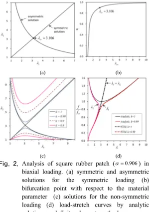
(λ1−λ2 λ14λ42−λ12−λ22−λ1λ2 α− + λ31λ23+ α = (16) Equation (16) gives two solutions. The one is symmetric deformation λ = and the other is 1 λ2 asymmetric deformation that can be solved by numerical method. Fig. 2(a) shows the symmetric and asymmetric solution for α=0.906 that was used for experimental verification for the Kearsley's bifurcation[15]. Letting λ=λ1=λ2 for the symmetric solution, bifurcation point can be determined by solving the following equation
0 ) 1 ( ) 1 )(
3
(λ8− λ2 α− + λ6+ α= (17)
Fig. 2(b) shows the solution of equation (17), i.e., λcr
λ= with respect to the specific material parameter
α
. Bifurcation point for the example material (α=0.906) is λcr=3.106 as derived in the literature[15].For asymmetric loading k<1, equation (15) can be written as
α λ λ λ λ λ λ α
λ λ λ λ λ
λ )( 1) ( )
(k 14 52− 15 24+ 31−k 13 − + k 14 32− 13 24+ 1−k 2
=0 (18)
Solution of equation (18) is shown in Fig. 2(c) where various =k 1, 0.99, 0.9 and 0.8 are compared.
For k=1 and 0.99, equation (14a) and 14(b) give load versus stretch curves resulting Fig. 2(d). In this
work, the same value for the bifurcation load 12
.
=23
fcr N is obtained as in the literature[15]. In Fig. 2(d), finite element method solutions are plotted along with the analytic solutions and their results are almost identical. One hundred linear quadrilateral plane stress elements are used for the solution.
f1
f2
f1
f2
F1
F2
(a) (b) (c)
Fig. 1. Square rubber patch. (a) uniformly distributed biaxial edge loading (b) 10x10 finite element model with distributed loading control (c) 10x10 finite element model with constrained edge loading
(a) (b)
(c) (d)
Fig. 2. Analysis of square rubber patch (α=0.906) in biaxial loading. (a) symmetric and asymmetric solutions for the symmetric loading (b) bifurcation point with respect to the material parameter (c) solutions for the non-symmetric loading (d) load-stretch curves by analytic solutions and finite element methods
Obtaining load-stretch behaviors by the finite element methods needs special considerations with care for it may lead to be unstable. For example, in loading
control such as in Fig. 1(b), general static analysis by incremental method with Newton-Rhapson iterations can be done for most increments but some increments may diverge due to excessive oscillatory iterations by numerical truncation error. It is typical for membrane analysis with rubber-like materials. One remedy for such a numerical instability is to model constrained edges as in Fig. 1(c) where the same displacement constraints are imposed along each edge and impose resultant load instead of distributed load.
For symmetrically loaded square patch, that is f
f
f1= 2= , bifurcation point should be found by the finite element method using linear perturbation and eigenvalue analysis. At bifurcation point, tangent stiffness matrix Kt becomes singular, i.e., Kt⋅u=0 for nontrivial displacement solution
u
. Referring to base state at load f0<fcr before singular point load f , crone can set up the following eigenvalue problem by applying perturbation load fΔ onto the base state
0 )
(K0+ηΔK ⋅u = (19)
where η is an eigenvalue, f~cr=f0+ηΔf is the estimated bifurcation load, K0=K0(f0) is the stiffness matrix at base state, ΔK=ΔK( fΔ ) is the differential stiffness matrix by perturbation of incremental loading Δ . Calculated bifurcation points are listed in Table 1 f for the square rubber patch for Fig. 1(a) with example material[14]. As shown in the table, bifurcation point can be identified however its value is not accurate but approximate especially at base state long before the bifurcation point. It is certain that the material nonlinearity affects the stiffness matrix that becomes singular approaching bifurcation point. By this investigation, in the context of finite element methods, even though general nonlinear analysis such as Fig.
2(d) is very accurate, finding bifurcation points of rubber-like materials using eigenvalue analysis cannot be recommended as a robust technique.
Existence of Kearsley's bifurcation phenomena for
square patch with Mooney-Rivlin material was verified by the experiment[15] and by the analytical or numerical method. In this study other material models described in the previous section will be investigated next. Neo-Hookean material (7) can be treated as α=1 by Mooney-Rivlin material. For α=1, there is no asymmetric solution from equation (16). It means
∞
cr→
λ as α→1 from Fig. 2(b). Therefore bifurcation cannot happen by neo-Hookean models.
For Gent material (11), equation (15) can be written
2 0
1 4 2 3 1 3 2 4
1λ −λλ +λ− λ =
λ k
k (20)
Equation (20) for symmetric loading, k=1, is
0 ) 1 )(
1 )(
(λ1−λ2 λ1λ2+ λ12λ22−λ1λ2+ = (21) This means that there is only one symmetric solution so the bifurcation cannot be observed for the Gent model. Likewise, Arruda-Boyce (9) and Fung model (12) are investigated by the same procedure and verified that there is no bifurcation or asymmetric deformation for the symmetric loading. For Pucci-Saccomandi model (13) in which strain energy density is dependent on I2 as well as I1, equation (20) for symmetric loading, k=1, can also be written
0 ) , , , ( )
(λ1−λ2 hλ1λ2 Jm β = (22)
where function h(λ1,λ2,Jm,β) has no real solution meaning no bifurcation phenomenon. Among material models described in the section 2.2, it is concluded that Kearsley's bifurcation occurs only for Mooney-Rivlin model.
Table 1. FEM calculation of bifurcation point using base state and eigenvalue analysis with perturbation fcr
f /0 0.5 0.6 0.7 0.8 0.9 0.95 0.99 1.01 1.1
cr cr f
~f /
0.6194 0.7051 0.7853 0.8608 0.9322 0.9666 0.9935 * *
*) eigensolution cannot be found due to numerical singularities at the base state
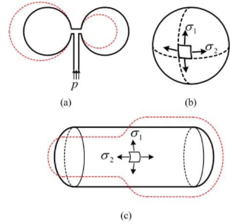
3.2 General inflation of rubber balloons Rubber balloons are easily inflated but may exhibit various kinds of instabilities. For example, there may be possible either symmetric or asymmetric inflation of symmetrically pressurized twin rubber balloons of Fig.
3(a). One balloon becomes larger while the other balloon becomes smaller at some point during inflation.
It is because of the existence of limit point that is caused by the rubber material and the geometry of the balloon. Likewise, even single balloon such as Fig.
3(b) and (c) may exhibit bifurcation or instability during inflation.
Both spherical and cylindrical balloon can be expressed by the following general inflation equation:
2 0
1− =
⋅σ σ
κ (23)
Stresses σ1 and σ2 in equation (23) are membrane stresses in zenith and azimuth direction respectively as shown in Fig. 3(b) and (c). For spherical balloon,
=1
κ
, and for cylindrical balloon, κ=1/2. For a specific material of section 2.2, stresses are defined by equations (6b) and (6c) assuming plane stress condition3=0
σ and incompressibility λ3=(λ1λ2)−1. Then, by solving equation (23), it can be obtained as λ1=λ1(λ2) or λ2=λ2(λ1). Inflation pressure is then recovered by,
0 1 0 0 2 2 1
1 0 1
r t r t r p t
⋅
= ⋅
= ⋅
= ⋅
υ σ λ λ
σ σ
(24)
where, r=λ1r0, t=t0/λ1λ2, υ=λ12λ2 are used and r0, t0 are initial radius, initial thickness, respectively.
Parameter υ is introduced to indicate a level of inflated volume. Internal pressure can be expressed in dimensionless form as follows:
G G t
p r
υ
ϕ σ1
0
0 =
= (25)
σ1
σ2
p
(a) (b)
σ1
σ2
(c)
Fig. 3. Rubber balloons inflations. (a) two balloons inflating by the same inflation pressure (b) spherical(ball) balloon inflation (c) cylindrical (tube) balloon inflation
Equation (23) and then (25) can be solved analytically for simple material models such as neo-Hookean or Gent model[7]. For neo-Hookean model it can be found as:
1 )
( 1− 7 1/3 =
= υ− υ− κ
ϕ for (26a)
2 / 1 1
2 1 1
3 / 1
2
2 ⎟ =
⎠
⎜ ⎞
⎝
⎛
⎟ +
⎠
⎜ ⎞
⎝⎛ −
= κ
υ υ
ϕ υ for (26b)
Equation (26a) and (26b) are plotted in Fig. 4(a) and 4(b). Other models are plotted as well in the same figure with the values of specific material constants. As shown in the figure neo-Hookean model shows a limit point but no stiffening beyond the limit point. It means balloon turns into very large inflation that is burst of the balloon.
For neo-Hookean model limit point is 620
. 0 , 64 . 2 7
2 = =
= ϕ
υ for ball balloon and
750 . 0 , 93 . 2 21
4+ = =
= ϕ
υ for tube balloon,
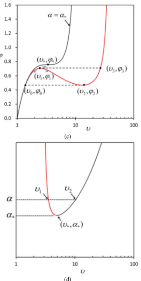
respectively. For other models, limit points are listed in Table 2 and 3. There is another limit point beyond the first limit point as shown in Fig. 3(c). For certain material constant, there is no limit point at all. For example, ball balloon of Mooney-Rivlin model, equation (8), has no limit point when α<α*=0.82. So
a critical material constant, i.e., (⋅ that divides stable )* and unstable inflation of the balloon can be identified as shown in Fig. 3(c). In Table 2 and 3 α*, J , m* λm* and b* represent those critical material constants. Fig.
4(d) is used to find critical material parameters. Lower α*
α < has no limit point at all meaning there is no instability or softening during inflation. Other points including the first (υ1,ϕ1) and the second (υ2,ϕ2) limit points are depicted in Fig. 4(c) and are listed in Table 2 and 3. In Fig 4(c), point '0' is the point of the same pressure with the second limit before the first limit point. Likewise, point '3' is the point of the same pressure with the first limit after the second limit point.
(a)
(b)
(c)
(d)
Fig. 4. Inflation curves. (a) ball balloon (b) tube balloon (c) inflation paths (d) critical material parameter.
NH: neo-Hookean, MR: Mooney-Rivlin, GE:
Gent, GE2: Gent or Pucci and Saccomandi, FU:
Fung, AB: Arruda-Boyce
Table 2. Inflation characteristics for spherical balloon (κ=1) Material
models
Material
constants (υ*,ϕ*) (υ1,ϕ1) (υ2,ϕ2) (υ3)(υ0)
NH (2.65, .620) (∞, 0)
MR α*= .824 (6.20, .752)
α= .906 (3.25, .680) (29.2, .583) (163) (1.75)
GE Jm*= 17.6 (4.43, .675)
Jm= 30.0 (3.02, .646) (12.5, .579) (27.7) (1.81) GE2
m*
J = 14.1 (4.10, .692)
β=0.9 Jm= 30.0 (2.80, .655) (14.1, .543) (30.8) (1.62) AB
m*
λ = 2.26 (4.29, .670)
λm= 3 (2.92, .640) (14.1, .550) (31.4) (1.69)
FU b*= .067 (4.86, .783)
b= .050 (3.33, .732) (10.4, .697) (20.1) (2.17)
Table 3. Inflation characteristics for cylindrical balloon (κ=0.5) Material
models α* (υ*,ϕ*) (υ1,ϕ1) (υ2,ϕ2) (υ3) (υ0)
NH (2.93, .750) (∞, 0)
MR α*= .5 (∞, 1)
α= .906 (3.51, .800) (∞, .584) (1.57) GE Jm*= 18.2 (5.00, .818)
Jm= 30.0 (3.38, .784) (13.5, .708) (26.7) (2.00) GE2 Jm*= 15.1 (4.70, .830)
β=0.9 Jm= 30.0 (3.21, .786) (15.2, .665) (32.4) (1.80) AB λm*= 2.29 (4.84, .812)
λm= 3 (3.26, .776) (15.2, .674) (33.4) (1.85) FU b = .065* (5.50, .946)
b = .050 (3.78, .889) (11.2, .853) (20.87) (2.47)
3.3 Bifurcation of rubber balloons
Using Table 2 and 3, bifurcation of twin ball balloons of Fig. 3(a) and a tube balloon of Fig. 3(c) can be identified. Considering twin ball balloons of Arruda-Boyce model with λm=3 inflated by blowing air into up to the first limit point, (υ1,ϕ1)= (2.92, .640) as listed in Table 2, the balloon will be inflated either symmetric or asymmetric fashion. Symmetric fashion occurs if both balloons are inflated up to point 3 in Fig. 4(c) meaning enough air as large as υ3= 31.4 is blown into the balloons while maintaining pressure as ϕ3=0.640. Asymmetric fashion occurs if one balloon is inflated up to point 2 while the other balloon shrinks back to point 0 meaning the pressure is dropped to ϕ0=ϕ2= 0.550. Volume and size of the balloons are calculated noting that 2 2
1
0 λλ
υ= VV = .
υ
=
= 3
0 3
0 r
r V
V
(27a)
03 . 69 2 . 1
1 .
314
3 0
2 = =
= υ υ
a b
r r
(27b)
where r and 0 r are initial and inflated radius, ra and
r
b represent radius of the smaller and the largeballoons when asymmetric inflation occurs.
Asymmetric inflation is depicted as dashed line in Fig.
4(a).
Likewise tube balloon may exhibit asymmetric inflation. From Table 3, Arruda-Boyce model of
=3
λm their values are (υ1,ϕ1)=(3.26, .776), )
,
(υ2 ϕ2 =(15.2, .674), υ0=1.85 and υ3=33.4. From equation (23), it can be found that λ1=1.32 and λ2
=1.06 at point 0 while λ =2.78 and 1 λ =1.97 at point 2.2
υ
=
=
0 2 0 2
0 l
l r r V V
(28a)
10 . 85 2 . 1
2 . 15 97 . 1
06 . 1
0
2 = =
= υ
υ λ λ
b a a b
r r
(28b)
Where l0 and l are initial and inflated tube lengths, ra and rb represent radius of the smaller and the large balloons, λa and λb represent axial stretch of the smaller and the larger balloon. Furthermore in a single tube balloon, asymmetric inflation can be occurred and is depicted as dashed line in Fig. 4(c).
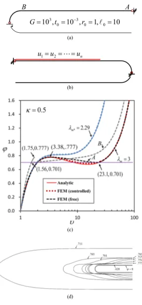
Asymmetric inflation analyses can be done by finite element method. Consider the aforementioned tube balloon of Arruda-Boyce rubber material. Tube balloon is modeled by axisymmetric finite elements as shown in Fig. 5(a) and (b) where boundary conditions, dimensions and material properties are listed. There is no restraint imposed between the point A and B in the model Fig. 5(a) while constraint equation of equal radial displacement is imposed for about two thirds of the tube wall in the model Fig. 5(b). Elemental length is 0.1 and the total of 120 linear axisymmetric shell elements are used. Riks method or arc-length method should be used to capture limit points and bifurcation phenomenon where either stable or unstable equilibrium path can be traced using material nonlinearity and large geometry.
At first, material with λ=λm*= 2.29 listed at Table
3 is analyzed by the model Fig. 5(a). Finite element result is drawn in Fig. 5(c) by blue dots showing that the result coincides with the analytic result obtained from the previous section. Secondly, material with λm
= 3 listed at Table 3 is analyzed by the model Fig.
5(b). Here Fig. 5(b) should be used to control equilibrium path of uniform inflation rather than that of bifurcated inflation. Finite element result is drawn in Fig. 5(c) by red dots as labeled 'controlled' showing that the result almost coincides with the analytic result obtained from the previous section. Note that slightly higher solution is obtained due to the constraints imposed along tube wall.
Lastly, material with λ = 3 is analyzed by the m
model Fig. 5(a) where tube wall is free to inflate in any direction. Finite element results are drawn in Fig.
5(c) by dashed lines as labeled 'free' showing the equilibrium path is bifurcated. Portion of tube containing point A in Fig. 5(a) bifurcate from the limit point (υ1,ϕ1)=(3.38, .777) to the point (υ3,ϕ3)=(23.1, .701). Portion of tube containing point B in Fig. 5(a) bifurcate from the limit point (υ1,ϕ1)=(1.75, .777) to the point (υ0,ϕ0)=(1.56, .701). This bifurcated inflation pattern is plotted in Fig. 5(d). See inflated shape at ϕ=.777 and ϕ=.701 in Fig. 5(d) those are limiting instances. Note that those results are slightly different from the analytic results in Table 3. It is for the geometric imperfection is inherent in the finite element model Fig. 5(a). At bifurcated instance, the ratio of larger to smaller radius, equation (28b), was 2.10 from the previous analysis. By the finite element method, it is calculated as follows:
64 . 56 2 . 1
1 . 23 27 . 2
07 . 1
0
2 = =
= υ
υ λ λ
b a a b
r r
(29)
Again, the result is slightly different from the analytic result because of the imperfection in the model of Fig. 5(a). From Fig. 5(d), note that the pressure at
fully inflated instance is ϕ=.711 whose value is much smaller than ϕ=.777 of pre inflated instance. This explains why at certain point of blowing the balloon is inflating so fast. That is the everyday practice when we are blowing many tube balloons for parties and fun.
10 , 1 , 10 ,
103 0= 3 0= 0=
= t − r l
G
A B
(a)
un
u u1= 2=L=
(b)
(c)
(d)
Fig. 5. Tube balloon inflation and bifurcation. (a) ax-isymmetric FEM model with no restraint for inflation (b) axisymmetric FEM model with restraint for infla-tion (c) analytic results and FEM results (d) inflation and bifurcation instances of tube balloon.
3. Conclusion
Inflation and bifurcation behaviors are analyzed for several typical hyper-elastic material models and key characteristics of the symmetric and asymmetric deformations are identified and estimated. Material models such as neo-Hookean, Mooney-Rivlin, Gent, Arruda-Boyce, Fung, and Pucci-Saccomandi are covered in this study. Analytic results are obtained by solving the general membrane equations while finite element results are obtained by using plane stress membrane elements and axi-symmetric shell elements.
Findings and remarks are summarized as follows:
1) For Treloar's patch problem, both from the analytic solutions and the finite element solutions, Mooney-Rivlin model shows the Kearsley's bifurcation phenomena while other models adopted in this study do not.
2) Physically this means it is very crucial that which model has to be used for certain type of problems when one needs to model rubber-like structures.
3) Finite element method gives accurate solution for load-displacement tracing if Newton's method with Riks or arc-length option is used. However finding bifurcation point, in this case due to the material stiffness, by finite element method with perturbed eigenvalue option is possible but not robust so it is not recommended.
4) Note that bifurcation problem due to the geometric stiffness such as buckling of the structures are solved by perturbed eigenvalue analysis and it is robust.
5) General inflation equation is solved analytically for the spherical and cylindrical balloons. By this study key characteristics such as critical material parameters and distinct limit points are identified.
6) Bifurcation characteristics of twin ball or tube balloons are estimated by those key characteristics.
7) Finite element solutions for the tube balloon which shows symmetric and asymmetric inflation are compared with those of analytic solution. Special
consideration when modeling tube balloon by finite element method is suggested.
References
[1] R. Mangan, M. Destrade, “Gent models for the inflation of spherical balloons”, International Journal of Non-Linear Mechanics, Vol. 68, pp. 52-58, 2015.
DOI:https://dx.doi.org/10.1016/j.ijnonlinmec.2014.05.016 [2] M. A. Destrade, A. Ni Annaidh, C. D. Coman, “Bending
instabilities of soft biological tissues”, International Journal of Solids and Structures, Vol. 46, No. 25-26, pp.
4322-4330, 2009.
DOI:https://dx.doi.org/10.1016/j.ijsolstr.2009.08.017 [3] D. R. Merritt, F. Weinhaus, “The pressure curve for a
rubber balloon”, American Journal of Physics, Vol. 46, No. 10, pp. 976-977, 1978.
DOI:https://dx.doi.org/10.1119/1.11486
[4] M. S. Park, S. Song, “Comparative study of bifurcation behavior of rubber in accordance with the constitutive equations”, The Korean Society of Mechanical Engineers, Vol. 34, No. 6, pp. 731-742, 2010.
DOI:https://dx.doi.org/10.3795/KSME-A.2010.34.6.731 [5] L. R. G. Treloar, “The elasticity and related properties of
rubbers”, Reports on Progress in Physics, Vol. 36, No.
7, p. 755, 1973.
DOI:https://dx.doi.org/10.1088/0034-4885/36/7/001 [6] A. N. Gent, I. S. Cho, “Surface instabilities in
compressed or bent rubber blocks”, Rubber Chemistry and Technology, Vol. 72, No. 2, pp. 253-262, 1999.
DOI:https://dx.doi.org/10.5254/1.3538798
[7] L. M. Kanner, C. O. Horgan, “Elastic instabilities for strain-stiffening rubber-like spherical and cylindrical thin shells under inflation”, International Journal of Non-Linear Mechanics, Vol. 42, No. 2, pp. 204-215, 2007.
DOI:https://dx.doi.org/10.1016/j.ijnonlinmec.2006.10.010 [8] A. Gent, “A new constitutive relation for rubber”, Rubber
chemistry and technology, Vol. 69, No. 1, pp. 59-61, 1996.
DOI:https://dx.doi.org/10.5254/1.3538357
[9] E. M. Arruda, M. C. Boyce, “A three-dimensional constitutive model for the large deformation stretch behavior of rubber elastic materials”, Journal of the Mechanics and Physics of Solids, Vol. 41, pp. 389-412, 1993.
DOI:https://doi.org/10.1016/0022-5096(93)90013-6 [10] C. O. Horgan, G. Saccomandi, “A molecular-statistical
basis for the Gent constitutive model of rubber elasticity”, Journal of Elasticity, Vol. 68, pp. 167-176, 2002.
DOI:https://doi.org/10.1023/A:1026029111723
[11] Y. C. Fung, “Elasticity of soft tissues in simple elongation”, The American journal of physiology, Vol.
213, No. 6, pp. 1532-1544, 1967.
DOI:https://dx.doi.org/10.1152/ajplegacy.1967.213.6.1532
[12] E. Pucci, G. Saccomandi, “A note on the gent model for rubber-like materials”, Rubber Chemistry and Technology, Vol. 75, No. 5, pp. 839-851, 2002.
DOI: https://dx.doi.org/10.5254/1.3547687
[13] A. N. Gent, “Elastic Instabilities in Rubber”, International Journal of Non-Linear Mechanics, Vol. 40 pp. 156-175, 2005.
DOI:https://dx.doi.org/10.1016/j.ijnonlinmec.2004.05.006 [14] E. A. Kearsley, “Asymmetric stretching of a
symmetrically loaded elastic sheet”, International Journal of Solids and Structures, Vol. 22, pp. 111-119, 1985.
DOI: https://dx.doi.org/10.1016/0020-7683(86)90001-6 [15] R. C. Batra, I. Mueller, P. Strehlow, “Treloar's biaxial
tests and Kearsley's bifurcation in rubber sheets”, Mathematics and Mechanics of Solids, Vol. 10, No. 6, pp. 705-713, 2005.
DOI: https://dx.doi.org/10.1177/1081286505043032
Moon-Shik Park [Regular member]
•Feb. 1989 : KAIST, MS
•Aug. 1994 : KAIST, PhD
•Aug. 1994 ∼ Feb. 1999 : Daewoo Heavy Industries, Chief Engineer
•Feb. 1999 ∼ current : Hannam Univ., Dept. of Mech. Eng., Professor
<Research Interests>
Multi-scale modeling and analysis of composite structures Theory of strain gradient plasticity and analysis
Rubber and polymer materials constitutive equations and bifurcation analysis
Transient response analysis and response spectrum analysis (DDAM, DAA)