THE DEVELOPMENT OF IR-BASED VISIBLE CHANNEL CALIBRATION USING DEEP CONVECTIVE CLOUDS
Seung-Hee Ham and Byung-Ju Sohn
Seoul National University
ABSTRACT: Visible channel calibration method using deep convective clouds (DCCs) is developed. The method has advantages that visible radiance is not sensitive to cloud optical thickness (COT) for deep convective clouds because visible radiance no longer increases when COT exceeds 100. Therefore, once DCCs are chosen appropriately, and then cloud optical properties can be assumed without operational ancillary data for the specification of cloud conditions in radiative transfer model. In this study, it is investigated whether IR measurements can be used for the selection of DCC targets. To construct appropriate threshold value for the selection of DCCs, the statistics of cloud optical properties are collected with MODIS measurements. When MODIS brightness temperature (TB) at 11 μ m is restricted to be less than 190 K, it is shown that more than 85% of selected pixels show COT ≥ 100. Moreover, effective radius (r e ) distribution shows a sharp peak around 20 μm. Based on those MODIS observations, cloud optical properties are assumed as COT = 200 and r e = 20 μm for the simulation of MODIS visible (0.646 μm) band radiances over DCC targets.
KEY WORDS: Deep convective cloud, vicarious calibration, visible sensor 1. INTRODUCTION
For obtaining accurate atmospheric, surface, and oceanic parameters from satellite observations, radiometric calibration should precede retrieval processes (Sohn et al., 2008). Absolute calibration converts observed digital counts into radiance quantities (W m -2 sr -
1 μm -1 ) which are treated in most of retrieval algorithms and analysis of radiation budget. As there is a linear relationship between digital counts and radiances for the visible spectral region, calibration coefficient can be defined as a proportional constant.
Vicarious calibration is performed apart from onboard calibration and this provides opportunity to evaluate onboard calibration system. Theoretically-estimated radiance values are simulated using radiative transfer model (RTM) and then calibration coefficient can be derived from regression between observed digital counts and simulated radiances.
As a calibration target, optically thick cloud has several advantages because atmospheric and surface effects can be minimized on the top-of-atmosphere (TOA) radiances.
Therefore, climate data can be used for the specification of atmospheric and surface conditions in the RTM. In addition, if we only consider deep convective clouds (DCCs) whose optical thickness is greater than 100, accurate cloud optical properties would be not needed in the modelling because visible reflectance is insensitive to COT. Therefore, cloud conditions will be assumed with reasonable accuracy for the simulation of visible radiances and then visible sensor will be calibrated. The developed calibration method will be applied to well- calibrated MODIS sensor for the assessment of the algorithm.
2. RADIATIVE TRANSFER SIMULATION OF VISIBLE BAND FOR THE CLOUD TARGETS 2.1 Radiative transfer model
The Discrete Ordinates Radiative Transfer (DISORT) (Stamnes et al., 1988) model is used as RTM to simulate TOA radiances in cloudy atmosphere. The model considers multiple scattering by atmospheric particles such as molecule, aerosol, and cloud particles.
Ice bulk scattering properties (Baum et al., 2005a and 2005b) based on theoretical scattering computations (Yang et al., 2003) and in-situ microphysical data are used to describe cloud optical properties in the RTM.
Note that only ice optical properties are considered in this study because DDC tops are generally located above tropopause layer and therefore, upper layers of DCCs are mostly composed of nonspherical ice particles.
In the simulations, cloud top height (CTH) is assumed to be 15 km. Moreover, based on the analysis with CloudSat measurements, it is found that geometrical depths of DCCs are normally greater than 10 km (Chung et al., 2008), and therefore, cloud base height is set by 1 km. Atmospheric profiles are assumed from standard tropical profiles.
In order to simulate sensor-reaching radiances, satellite viewing zenith angle (VZA), viewing azimuth angle (VAA), solar zenith angle (SZA) and solar azimuth angle (SAA) are input to the RTM.
2.2 Possible use of DCCs for the visible channel calibration
Relationships between COTs and visible flux
reflectances are obtained from model simulation in Figure
1. Fixed effective radius of 20 μm is used. Flux
reflectances increase as COT increases, but the slope
decreases. As a result, when COT exceeds 200, reflectance is almost constant with COT.
To quantify those effects of COT on visible reflectances for various viewing geometries, TOA bidirectional reflectance distribution functions (BRDFs) are simulated with three COT values (= 100, 200, and 400) while r e = 20 μm. For the given COT, bidirectional reflectances are calculated for various viewing geometries (0° ≤ VZA≤ 60° and 0° ≤ RAAs ≤ 180°) while SZA is fixed as 30°. Upper panels of Figure 2 show simulated TOA BRDFs. Radial axis means VZA (θ v ) and tangential axis means RAA (φ ). It seems that angular distribution of reflectances is less affected by COT, but small biases between BRDFs for different COTs are found. The differences of BRDFs between COT = 100 vs.
COT = 200 and COT = 200 vs. COT = 400 are also given on the lower panels in Figure 2. The maximum difference of BRDFs is 0.05 (0.025) when COT increases from 100 to 200 (from 200 to 400).
In conclusion, minor variations of visible reflectances are noted by change of COT for DCCs. This suggests that visible reflectances can be simulated accurately with fixed cloud optical properties. If we assign those cloud parameters based on the observation, operational ancillary data are not need for the specification of cloud properties in the RTM.
3. THE USE OF IR MEASUREMENTS FOR THE SELECTION OF DCC TARGETS
Over the tropical latitudes, there are abundant clouds overshooting the tropical tropopause layer (TTL). Those DCCs generally show cold TB 11 values less than 190 K in the center of convective systems. This suggests that cloud top signals tend to be colder than tropopause temperatures.
These cold signals can be explained by adiabatic cooling at cloud tops. DCCs involve strong upward motion lacking of exchange with ambient air (Lattanzio et al., 2006). As a result, even after passing TTL, Cloud top temperature (CTT) keeps decreasing with height whereas environmental temperature increases. Therefore, low TB 11 values are likely to be appeared near core regions of DCCs overshooting TTL. Note that thin cirrus located near TTL generally represents higher TB 11 value compared to DCC (i.e., TB 11 > 190 K) because warm signal near the surface can penetrate cirrus and also reach to the satellite sensor.
The utility of TB 11 for the selection of DCC targets is examined by collecting statistics of MODIS measurements obtained in January 2006 over the low- latitude region (40°S−40°N, 180°W−180°E). Figure 3 shows histograms of 0.646 μm reflectances (=
πR0.646/F 0 cosθ 0 ), COT, and r e of the MODIS pixels satisfying following conditions:
TB 11 ≤ 190 K (1)
STD of TB 11 for 81 (9 × 9) pixels within a grid box centered on the pixel ≤ 1 K (2)
where TB 11 is obtained from MODIS band 31 (11.026 μm) measurements.
Horizontal homogeneous condition given in equation (2) is applied for the elimination of edge pixels showing rapid change of cloud top height (CTH). Most of selected pixels show high reflectance values (> 0.9), implying that optically thick clouds exist. On the other hand, about 85.7% of pixels show COT values as 100. Considering that MODIS cloud algorithm retrieves COT up to 100, actual COT could be much larger than 100 in this case.
Remained 14.3% pixels represent small COT values (<
100) which are likely to be appeared in edge area of DCC although the equation (2) is applied. On the other hand, histogram of effective particle radius shows maximum frequency at 19 μm (i.e., mode radius) and mean effective radius is 20.61 μm.
4. CALIBRATION OF VISIBLE BANDS OVER DCC TARGETS
Weak dependence of visible reflectances on COTs proposes that visible band reflectances can be simulated accurately with assumed cloud parameters for the case of DCCs. With those assumed cloud parameters (i.e., COT = 200 and r e = 20 μm), visible band radiances can be simulated and then calibration coefficient can be derived by regression between detected digital counts and simulated radiances.
In this study, MODIS visible band (0.646 μm) radiances are simulated and then compared observed radiances. This can provide an opportunity to evaluate the accuracy of developed calibration algorithm because MODIS sensor equipped onboard calibration system and therefore those bands are well calibrated.
Six month MODIS data (January to June 2006) on Aqua platforms are considered for monitoring seasonal variations of calibration results. Scatter plots between simulated vs. observed MODIS band 1 (0.646 μm) reflectances are made in Figure 4. Although same cloud parameters are used for all pixels, most of pixels show less than 20% uncertainties through the entire period.
Only few pixels show large overestimation of reflectances compared to the observed values, particularly noted in April and May. Those overestimations are likely to be generated by the selection of edge pixels of DCCs. It has been discussed that 15% of selected cloud pixels could have small COT values when threshold conditions in equation (1) and (2) are used.
Daily mean values are calculated only if N pixel ≥ 10 where N pixel is the number of selected cloud pixels per day.
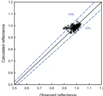
Scatter plots between simulated and observed mean values are presented in Figure 5. It is shown that most of points fall within the ±5% uncertainty lines (blue dashed lines) while only few points show more than 5%
overestimation.
5. CONCLUSIONS
• In the core regions of DCCs, TB 11 tends to be colder than tropopause temperature because of strong upward motion lacking of exchange with ambient air.
• If we choose cloud pixels when TB 11 ≤ 190K and STD of TB11 for 81 (9 × 9) pixels within a grid box centered on the pixel ≤ 1K, more than 85% of pixels are greater than 100.
• With assumed cloud parameters, MODIS visible band (0.646 μm) radiances are simulated. The comparison of simulated radiances with MODIS-observed radiances for half year of 2006 demonstrates that visible channel measurements can be calibrated within a ±5% uncertainty range on a daily basis.
References
Baum, B. A., A. J. Heymsfield, P. Yang, and S. T. Bedka, 2005a. Bulk scattering models for the remote sensing of ice clouds. Part 1: Microphysical data and models, J. Appl. Meteor., 44, 1885–1895.
Baum, B. A., P. Yang, A. J. Heymsfield, S. Platnick, M. D.
King, Y.-X. Hu, and S. T. Bedka, 2005b. Bulk scattering models for the remote sensing of ice clouds. Part 2:
Narrowband models, J. Appl. Meteor., 44, 1896–1911.
Lattanzio, A., Watts, P. D., and Govaerts, Y., 2006. Physical interpretation of warm water vapour pixels, report TM 14, 43 pp., EUMETSAT.
Sohn, B.-J., H.-S. Park, H.-J. Han, and M.-H. Ahn, 2008.
Evaluating the calibration of MTSAT-1R infrared channels using collocated Terra MODIS measurements. Int. J. Remote Sens., 29, 3033-3042.
Stamnes, K., S.-C. Tsay, W. J. Wiscombe, and K. Jayaweera, 1988. Numerically stable algorithm for discrete-ordinate- method radiative transfer in multiple scattering and emitting layered media. Appl. Opt., 27, 2502–2509.
Yang, P., B. A. Baum, A. J. Heymsfield, Y.-X. Hu, H.-L.
Huang, S.-C. Tsay, and S. A. Ackerman, 2003. Single scattering properties of droxtals. J. Quant. Spectros. Rad. Transfer, 79-80, 1159–1169.
Acknoledgements
The authors wish to thank Korean Geostationary program (COMS) granted by the KMA.
SZA=30, r
e=20 μm
COT
0 100 200 300 400
Flux Reflectance
0.0 0.2 0.4 0.6 0.8 1.0 1.2
ice (0.646 μm) water (0.646 μm)
Figure 1. Relationships between COTs and flux reflectances when SZA = 30°
Figure 2. Simulated TOA BRDFs of ice cloud for three COT values of 100, 200, and 400. Also differences of BRDFs are presented for COT = 100 vs. COT = 200 and COT = 200 vs.
COT = 400 on the lower panels.
Figure 3. Histograms of 0.646 μm reflectance (πR0.646/F 0 cosθ 0 ), COT, and re for selected cloud pixels.
Figure 4. Comparisons between simulated and observed MODIS band 1 (0.646 μm) reflectances for six months.
MODIS Band 1 (0.646 μm)
Observed reflectance
0.5 0.6 0.7 0.8 0.9 1.0 1.1 1.2
Calculated reflectance
0.5 0.6 0.7 0.8 0.9 1.0 1.1 1.2
-5%
+5%