♾
공간적 다기준평가 기법을 이용한 도시의 삶의 질 분석
전병운
1※A Spatial Multicriteria Analysis Approach to Urban Quality of Life Assessment
Byong-Woon JUN
1※ABSTRACT
A pixel-based approach to urban quality of life assessment can be regarded as a spatial decision problem under the condition of complexity because it searches the urban space for evidence of hot spots of quality of life based on multiple and differentially weighted evaluation criteria. Such an assessment involves inappropriate scaling of several incommensurate criteria, much unstructured subjectivity in the decision maker’s judgment, and the large data handling in a raster GIS environment. There is a need for identifying alternative approaches to tackle the ill-structured problem in urban quality of life assessment. In this context, this research proposes and implements a spatial multicriteria analysis approach to evaluate urban quality of life in a raster GIS environment. The implementation of this methodology is illustrated with a case study of the Atlanta metropolitan area. Results indicate that the proposed methodology may provide an alternative approach for evaluating the quality of life in an urban environment.
KEYWORDS: Spatial Multicriteria Analysis, AHP, Quality of Life
요 약
도시의 삶의 질 분석에 대한 화소기반 기법은 복잡성이라는 조건 하에서의 공간의사결정문제로 간주될 수 있다. 왜냐하면, 도시의 삶의 질 분석은 상이한 가중치가 부여된 여러 개의 평가기준에 기반을 두고 높은 혹은 낮은 수준의 삶의 질을 가진 지역을 도시공간에서 탐색하기 때문이다. 이 러한 도시의 삶의 질 분석에는 측정단위가 다른 여러 개의 평가기준들의 부적절한 스케일링, 평가 자의 판단에 있어서 비구조적인 주관성 그리고 래스터 GIS환경에서 대량의 데이타 처리 등과 같 은 어려움이 있다. 도시의 삶의 질 분석에 있어서 이러한 비구조적 문제를 해결하기 위한 대안적 인 접근방법의 개발이 필요하다. 이러한 점에서, 본 연구는 래스터 GIS 환경에서 도시의 삶의 질
2008년 10월 28일 접수 Received on October 28, 2008 / 2008년 11월 28일 수정 Revised on November 28, 2008 / 2008년 12월 11일 심사완료 Accepted on December 11, 2008
1 경북대학교 지리학과 Department of Geography, Kyungpook National University
※ 연락저자 E-mail : [email protected]
을 평가하기 위한 공간적 다기준평가 기법을 제안하고자 한다. 이러한 방법론은 애틀란타 대도시 권을 사례로 예시되어진다. 본 연구에서 사용된 방법론은 도시의 삶의 질을 평가하는데 있어서 새 로운 대안적인 접근방법으로 제시된다.
주요어: 공간적 다기준평가, 계층분석과정, 삶의 질
INTRODUCTION
Themes related to quality of life (QOL) in the city were prominent in urban geography in the 1980s. However, interest in QOL research has recently been revived in many areas such as public policy, urban geography, and planning (Massam, 2002;
Pacione, 2003; Randall and Morton, 2003).
Quality of life has often been used as a policy goal. Enhancing the QOL of people is the ultimate goal of public policy. Moreover, QOL rankings of cities in the era of globalization have played an important role in attracting capital and stimulating economic growth (Rogerson, 1999).
Although much QOL research has been conducted in the last three decades, recent studies address some methodological challenges (Randall and Morton, 2003; Jun, 2006a; Rinner, 2007). First, there is no consensus on the definition of QOL. In this paper, QOL refers to the level of well‐
being of people and the physical conditions in which people live, but there are a number of contrasting definitions of what QOL means. Whatever the definition of QOL, the common ground in the geographic literature is that QOL is defined by the individual, but formalized by the community (Cutter, 1985;
Myers, 1987; Randall and Williams, 2002;
Randall and Morton, 2003).
Second, there is no consensus on the
selection of QOL indicators. Up to this point, various criteria including objective, subjective, and perceptual indicators have been used in QOL evaluation (Bederman and Hartshorn, 1984; Randall and Morton, 2003).
In most previous studies, some objective indicators including income, housing, and education have frequently been employed for measuring QOL because these indicators are easily available and not questionable (Wallace, 1971; Smith, 1973; Liu, 1976).
Much QOL research has utilized only a set of demographic and socio‐economic indicators from census data (Liu, 1976;
Bederman and Hartshorn, 1984). With recent advances in satellite remote sensing and geographic information system (GIS) technologies, environmental indicators such as land use and cover, normalized difference vegetation index (NDVI), and surface temperature derived from remotely sensed images have been used in conjunction with socioeconomic indicators to take a more complete picture of QOL (Forster, 1983;
Weber and Hirsch, 1992; Lo and Faber, 1997; Mesev, 2003; Jun, 2006b, Li and Weng, 2007). More recently, environmental justice research has indicated that hazard‐related indicators such as potential risks from environmental hazards need to be included in urban QOL assessment (Jun, 2006b). It is also suggested that some indicators such as the cultural and artistic workforce, diversity of origin and sexual orientation, and housing
diversity can be considered in future QOL assessment (Florida, 2002). What is clear is that previous studies within the geographic information science (GIScience) research community evaluated urban QOL by integrating hazard‐related indicators and environmental indicators from satellite images with socioeconomic indicators from census data.
Third, there is no consensus on the processing of QOL indicators. A zone‐
based approach to data aggregation has been employed in most previous studies to characterize QOL because of its economical operation and computational feasibility (Jun, 2006a). However, this zone‐based approach has led to serious methodological difficulties such as the modifiable areal unit problem (MAUP) and the incompatibility problem in areal units (Can, 1992; Spiekermann and Wegner, 2000). As an alternative for the zone‐based data aggregation, a pixel‐based approach to data aggregation is often suggested to tackle these problems and to reveal the sub-unit variations of QOL indicators in areal units (Jun, 2006a).
A pixel-based approach to urban QOL assessment can be regarded as a spatial decision problem under the condition of complexity. In such an assessment, decisions about the allocation of urban space are made on the basis of multiple evaluation criteria with different weightings to search for evidence of hot spots of quality of life.
The urban QOL assessment procedure involves inappropriate scaling of several incommensurate criteria and much unstructured subjectivity in the decision maker’s judgment, and handles large data in
a raster GIS environment (Pereira and Duckstein, 1993; Jankowski, 1995;
Malczewski, 1999; Rinner, 2007). There is a need for identifying alternative approaches to tackle the ill‐structured problem in urban QOL assessment.
In this context, this research proposes and implements a spatial multicriteria analysis approach to evaluate urban QOL in a raster GIS environment. The literature related to spatial multicriteria analysis (SMA) is reviewed in the next section. The methodology is then introduced and followed by the results with a discussion of them. In the last section, concluding remarks and summary are described.
SPATIAL MULTICRITERIA ANALYSIS
Typically, a spatial multicriteria decision problem involves evaluation of a set of geographically defined alternatives based on the criterion values and the decision maker’s preferences with respect to a given set of multiple and conflicting evaluation criteria (Malczewski, 1999). In terms of GIS, the alternatives are represented as a composite set of various map layers with different criteria weights while the criteria are map layers. The alternatives are often evaluated by the decision maker on the basis of unique preferences along the relative importance of criteria. In order to obtain information for making the decision, both data on criterion values and the geographic locations of alternatives are analyzed with GIS and multicriteria decision making (MCDM) techniques. The integration of GIS and MCDM techniques can benefit from
each other (Jankowski, 1995; Malczewski, 1999; Thill, 1999; Malczewski, 2006). On the one hand, GISs provide the capabilities to acquire, store, retrieve, manipulate, and analyze spatially referenced data in a spatial decision making environment. On the other hand, the MCDM techniques provide a rich set of methods to structure decision problems, and to design, evaluate and prioritize alternative decisions. The integration of GIS and MCDM techniques plays an important role in supporting the decision maker in achieving greater effectiveness and efficiency of decision making while solving spatial decision problems. The term GIS‐based multicriteira decision analysis is often used to address such an integration of GIS and MCDM techniques for solving the spatial multicriteria decision problem. This term is synonymously used with spatial multicriteria analysis (Malczewski, 1999). In this regard, SMA can be thought of as a process that integrates and transforms spatially referenced data and the decision maker’s preferences to obtain information for decision making (Malczewski, 2006).
Based on the framework described by Malczewski (1999), the SMA can be structured into five major stages: problem definition, criterion generation, criterion standardization, criterion weighting, and criterion aggregation. In the problem definition stage, a spatial decision problem is identified and raw data are obtained and processed for further decision making. The criterion generation stage involves specifying a set of evaluation criteria. A criterion serves as some basis for a decision that can
be measured and evaluated (Eastman et al., 1995). Each criterion is represented as a map layer in the GIS database. There are two types of criteria: factors and constraints. A factor positively or negatively contributes to the alternatives under consideration while a constraint limits the alternatives. In the criterion standardization stage, the values contained in various criteria are transformed to comparable units.
Although a number of approaches such as deterministic, probabilistic, and fuzzy methods can be used to make the evaluation criteria commensurate, linear scale transformation has been frequently used in most previous studies because of its simple operation (Voogd, 1983; Massam, 1988;
Eastman et al., 1995). In the criterion weighting stage, the weights of relative importance are assigned to the evaluation criteria under consideration. The decision maker’s preferences are elicited by the derivation of weights. There are several criterion weighting procedures including ranking, rating, pairwise comparison, and trade‐off methods. These procedures have different advantages and disadvantages in terms of a number of factors such as ease of use, accuracy, degree of understanding on the part of the decision maker, the theoretical foundation, the availability of computer software, and use in a GIS environment (Malczewski, 1999). Some empirical studies indicate that one of the most effective techniques for spatial decision making is the pairwise comparison method (Banai, 1993; Eastman et al., 1995; Rashed and Weeks, 2003; Malczewski, 2006; Rinner, 2007). The pairwise comparison method
developed by Saaty (1980) is often known as the analytic hierarchy process (AHP).
Finally, the criterion values and the decision maker’s preferences are integrated to provide an overall assessment of the alternatives in the criterion aggregation stage. This is achieved by decision rules which allow for ordering the alternatives. Many decision rules can be used to handle the spatial multicriteria decision problem. These rules include simple additive weighting (SAW) methods, value/utility function approaches, AHP, ideal point methods, concordance methods, and fuzzy aggregation operations.
To select an appropriate decision rule for a given decision situation, the following several factors are taken into account:
characteristics of the decision problem, characteristics of the decision maker, and characteristics of the decision rule (Malczewski, 1999). Some previous studies suggest that one of the most widely used MCDM methods is the SAW method (Voogd, 1983; Carver, 1991; Eastman et al., 1995). The method is also known as weighted linear combination (WLC) method.
The SMA approach has been most often used for solving many spatial decision problems such as land suitability, plan/scenario evaluation, site search/selection, and resources allocation problems (Malczewski, 2006). However, only a handful of previous studies have applied the SMA approach for urban QOL evaluation. Can (1992) used generalized concordance analysis to evaluate the residential quality scores at the census track and block group levels in the city of Syracuse, USA. More recently, Rinner (2007) has adopted the combination
of geographic visualization tools with the AHP method to calculate composite urban QOL scores at the census tract level in the city of Toronto, Canada. The two previous studies employed a zone‐based approach to urban QOL assessment. The zone‐based approach has major methodological problems such as the MAUP (Can, 1992; Spiekermann and Wegner, 2000; Apparicio et al., 2008) and the incompatibility problem in areal units (Spiekermann and Wegner, 2000) as indicated in the previous section. To solve these problems, a pixel‐based approach to urban QOL assessment was suggested (Jun, 2006a). The pixel‐based approach allows for revealing the sub‐unit variations of QOL indicators in areal units.
Urban QOL assessment in a raster GIS environment can be thought of as a spatial multicriteria decision problem involving a large number of alternatives and combining objective and subjective information.
Different MCDM techniques such as generalized concordance analysis and AHP were used in the two previous studies. The major disadvantage of using these MCDM techniques is that their implementation in a raster GIS environment is computationally more intensive and impractical since these techniques require comparison across a large number of individual grid cells. To handle this problem, raster procedures for multicriteria evaluations were proposed by Eastman and his colleagues (1995). Such a SMA approach can deal with some methodological problems such as inappropriate scaling of several incommensurate criteria and unstructured subjectivity in the decision maker’s preference (Pereira and Duckstein,
FIGURE 1. Location of study area 1993) and integrate the subjective information provided by a decision maker and the objective information in the urban QOL assessment. A pixel-based SMA approach to urban QOL assessment is at the core of this paper.
DATA AND METHODS
The Atlanta, Georgia metropolitan area in the US was selected as a study area. In this research, the Atlanta metropolitan area denotes the ten‐county planning area of the Atlanta Regional Commission (ARC) as shown in FIGURE 1. As a major trade, service, and transportation center in the southeastern US, the Atlanta metropolitan area has experienced fast economic growth for the past 30 years. As a major manufacturing center in the South, the metropolitan area has also suffered from the dire degeneration of urban climate and air
quality. In particular, this metropolitan area has undergone urban warming and the increases in ozone and emission of volatile organic compounds (Lo et al., 1997). In addition, high levels of urban inequality based on racial segregation have been identified in the metropolitan area. Therefore, the metropolitan area lies in extreme racial and economic, and environmental inequality.
In such a paradoxical geography, an urban QOL was evaluated in this paper.
Three major data sets such as Landsat TM image, census data, and toxic release inventory (TRI) database were used in this study. From 2000 Landsat 5 TM image, three environmental variables such as land use and cover, normalized difference vegetation index (NDVI), and surface temperature were derived. A hybrid digital image classification and a modified version of the Anderson scheme of land use and land cover classification with mixed levels 1 and 2 were used to extract a land use and land cover map. This land use and land cover map had six classes such as the residential, commercial and industrial (urban use), grassland/pasture/cropland, forest, water, and barren classes. This map was then reclassified to exclude water and barren classes. The overall accuracy of the land use and land cover map was 87.5 percent which is enough for further application. The NDVI was quantified for each pixel from bands 3 and 4 of the Landsat TM image. The NDVI is a greenness measure. Its value ranges from ‐ 1 to +1 with increasing greenness. Surface temperature was quantified for each pixel from band 6 of the Landsat TM image
using the equations proposed by Wukelic et al. (1989) and Nichol (1994).
From 2000 Census data, four socioeconomic variables such as population density, per capita income, percent college graduates, and median home value were extracted at the census block group level which is the smallest enumeration unit with socioeconomic information available. From 2000 Census TIGER/Line file, the census block group boundary file was extracted.
From U.S. Environmental Protection Agency (EPA)’s 2000 TRI database, a hazard‐related variable, cumulative potential relative exposure to TRI facilities, was derived using the following equation (Cutter et al., 2001):
) 0 . 1 (
1
∑=
−
= n
j j
ij
i p
p
T CPE d
where CPEi is cumulative proximal exposure to population in census unit i from distance to facility j at locations 1 through n (total number of facilities); dij is distance from population i to facility j; Tj is distance at which exposure is negligible for facility j;
and p is rate of reduction of exposure at increasing distance from j. To reduce the analytical complexity, the TRI facilities with airborne emissions were extracted from the TRI database. The CPE was then multiplied by the relative potential risk score (RPRS) for each TRI facility which represents the magnitude and the relative toxicity of release from TRI facilities. Based on the weighted CPEs, a risk surface was finally generated. The TRI database that is a national database of industrial facilities releasing toxic and hazardous chemicals is a more reliable approximation of chronic toxic
release.
An overview of the methodological framework implemented for this research is illustrated in FIGURE 2. Three environmental variables from the Landsat TM image, a hazard‐related variable from the TRI database, and four socioeconomic variables from the census data were integrated into a spatial database for the urban QOL assessment in the Atlanta metropolitan area. Four socioeconomic variables such as population density, per capita income, median home value, and education level are on a per‐zone basis.
However, a hazard‐related variable such as risk surface and three environmental variables such as land use and land cover, NDVI, and surface temperature are on a per
‐pixel basis. These two analytical units are not compatible with each other. There is the spatial mismatch problem in analytical units among different data. To handle the spatial mismatch problem in analytical units, most previous studies adopted the zone‐based approach which aggregates per‐pixel data to zonal units (Weber and Hirsch, 1992; Lo and Faber, 1997; Park, 2006; Li and Weng, 2007; Apparicio et al., 2008). Although the zone‐based approach to data aggregation was frequently used in most previous studies because of its analytical simplicity, it has not only some methodological pitfalls such as the MAUP and the incompatibility problem in areal units, but also the unrealistic assumption that all the socioeconomic data are uniformly distributed throughout the census block group (Spiekermann and Wegner, 2000; Jun, 2006a). As an alternative to the zone‐based
FIGURE 2. Research methodology approach, a pixel‐based approach to data
aggregation was used in this research to reveal the sub‐unit variation in zonal units.
Four socioeconomic variables at the census block group level were spatially disaggregated into individual pixels. Two demographic variables are spatially extensive data while two economic variables are spatially intensive data with the same value in each part of a zone. Goodchild and Lam (1980) suggests that different interpolation methods need to be applied according to the nature of spatial data. Based on their suggestion, different methods were used to spatially disaggregate four socioeconomic variables into individual pixels. A spatial disaggregation model developed by Jun (2006c) was used to allocate two
demographic variables such as population density and percent of college graduates to individual pixels. This model was implemented by the following equation proposed by Mennis (2003):
ub b ubc
ubc N
P P = F *
where Pubc is population assigned to one grid cell of land use/cover class u in block group b and in county c; Fubc is total fraction for land use/cover class u in block group b and in county c; Pb is population of block group b; and Nub is the number of grid cells of land use/cover class u in block group b. The following equation was employed to compute the total fraction (Fubc):
]
[( * ) ( * ) ( * )
*
nb nc lb lc hb hc
ub uc
ubc D A D A D A
A F D
+
= +
where Fubc is total fraction of land use/cover class u in block group b and in county c;
Duc is population density fraction of land use/cover class u in county c; Aub is area ratio of land use/cover class u in block group b; Dhc is population density fraction of land use/cover class h in county c; Dlc is population density fraction of land use/cover class l in county c; Dnc is population density fraction of land use/cover class n in county c; Ahb is areal ratio of land use/cover class h in block group b; Alb is area ratio of land use/cover class l in block group b; and Anb
is area ratio of land use/cover class n in block group b. A geostatistical modeling method known as inverse distance weighting (IDW) was also used to interpolate two economic variables such as per capita income and median home value into each pixel.
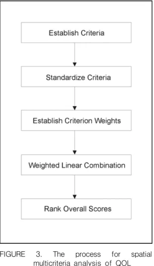
As illustrated in FIGURE 3, a SMA approach was developed in this research to integrate and transform environmental, hazard‐related, and socioeconomic variables into a resultant QOL score for each pixel.
The SMA process involves five main stages. The first stage is the selection of evaluation criteria or measures that determine the scope of the analysis as described in the previous section. The second stage is to standardize each criterion map layer through a linear scale transformation method based on the minimum and maximum values as expressed in the following equation:
) X (X
) X yi (xm a xi m i n
m i n
−
= −
where yi is the standardized score, xi is the raw value, Xmax is the maximum value, and Xmin is the minimum value. The value of standardized scores ranges from 0 to 1.
Because criteria are measured at the different scales, it is necessary that factors are standardized before combination. In the third stage, the evaluation criteria are compared pairwisely using the AHP developed by Saaty (1980) in order to generate the criterion weights. Although there are a variety of techniques for development of weights, Saaty’s AHP appears as one of the most promising (Eastman et al., 1995). The AHP approach allows one to assess the relative weight of multiple criteria in an intuitive manner. The weights sum to 1. In the fourth stage, the weighted standardized criteria are aggregated to generate the overall score using a decision rule based on a weighted linear combination (WLC) method. In the final stage, the overall performance scores are ranked into five ordinal levels by Jenks optimization method (Slocum et al., 2005).
As a spatial autocorrelation index, Moran’s I was used to measure the extent of spatial clustering among pixels in terms of QOL scores. To evaluate the performance of the SMA approach, the resultant QOL score map was statistically compared with the QOL score map generated by the principal components analysis (PCA) approach in the previous study (Jun, 2006b), which is an objective approach to urban
FIGURE 3. The process for spatial multicriteria analysis of QOL QOL assessment. A correlation analysis was performed to statistically verify the spatial similarity between the resultant QOL score map based on the SMA approach and the QOL score map generated by the PCA approach.
RESULTS AND DISCUSSION
1. Implementation
A SMA approach was developed to integrate and transform environmental, hazard‐related, and socioeconomic variables into a resultant QOL score for individual pixel. The SMA approach is the actual
decision making procedure of applying a decision rule to meet a specific objective on the basis of multiple and conflicting criteria (Malczewski, 1999). This approach is based on the integration of the WLC method along with the linear scale transformation method for normalizing the criteria and the AHP method for deriving the criterion weights.
Based on previous studies and data availability, the socioeconomic, environmental, and hazard‐related variables were selected to evaluate the QOL in the Atlanta metropolitan area in 2000. In most previous studies, the socioeconomic variables such as population density, percent college graduates, per capita income, and median home values have been commonly used as objective indicators for urban QOL assessment (Smith, 1973; Liu, 1976; Bederman and Hartshorn, 1984; Can, 1992; Pacione, 2003;
Randall and Morton, 2003). The environmental variables such as urban use, NDVI, and surface temperature derived from satellite imagery were included to provide a complete environmental perspective (Lo and Faber, 1997). A hazard‐related variable suggested by environmental justice research was adopted because this is an obvious factor of environmental disamenity in urban areas (Jun, 2006b). These variables are restructured into two major groups of factors. One is the positive factors such as NDVI, percent college graduates, per capita income, and median home values. In the positive factors, the higher values are more desirable to the QOL. The other is the negative factors such as urban use, surface temperature, cumulative potential relative exposure values to TRI facilities, and
LULC NDVI TEMP POPD EDU PINCO HOME RISK
LULC 1
NDVI 5 1
TEMP 5 1 1
POPD 1/5 1/7 1/5 1
EDU 3 1/3 1/3 5 1
PINCO 5 3 3 7 3 1
HOME 5 3 3 7 3 1 1
RISK 7 5 5 9 5 5 3 1
LULC - Urban use; NDVI - NDVI; TEMP - Surface temperatures; POPD - Population density;
EDU - Percent college graduates; PINCO - Per capita income; HOME - Median home value;
RISK - Cumulative potential relative exposure.
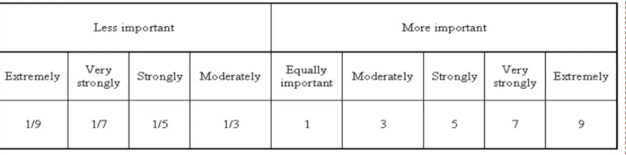
TABLE 1. A pariwise comparison matrix for assessing the relative importance of factors FIGURE 4. The continuous rating scale used for AHP pairwise comparison
population density. In the negative factors, the higher values are less desirable to the QOL.
Because the eight criteria are measured at the different scales, it is necessary that these criteria are standardized before combination. The eight factors were standardized to a consistent numeric range of 0 to 1. Standardization was achieved by undertaking a linear scale transformation method based on the minimum and maximum values as expressed in the previous section. Because of its economical operation, this method has been often used in most previous studies (Voogd, 1983;
Massam, 1988; Eastman et al., 1995;
Malczewski, 1999). In case of the negative factors, the numeric scales were reversed to reflect the undesirability to the QOL.
In the next stage, the AHP developed by Saaty (1980) was used to generate the criterion weights based on the pairwise comparison among the eight criteria. The AHP method is one of the most widely used multicriteria evaluation methods (Malczewski, 1999). The method assists the decision maker in eliciting his/her preferences by assessing the relative weights of multiple criteria in an intuitive manner. In the AHP method, the weights can be derived by taking the principal eigen vector of a square reciprocal matrix of
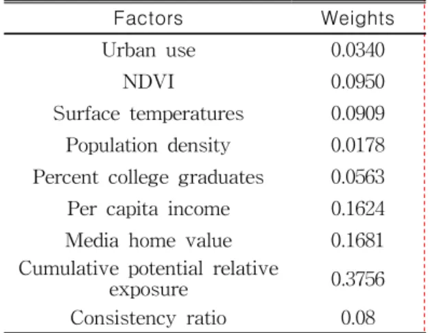
Factors Weights
Urban use 0.0340
NDVI 0.0950
Surface temperatures 0.0909 Population density 0.0178 Percent college graduates 0.0563 Per capita income 0.1624
Media home value 0.1681
Cumulative potential relative
exposure 0.3756
Consistency ratio 0.08
TABLE 2. Weights for factors and consistency ratio pairwise comparison. The comparisons
concern the relative importance of the two criteria involved in determining the QOL.
Ratings are provided on a nine‐point continuous scale as shown in FIGURE 4.
For example, if the analyst thought that NDVI was moderately more important than percent college graduates in determining the QOL, the analyst would enter a 3 on this scale. If the analyst thought that percent college graduates was moderately more important than NDVI, the analyst would enter 1/3. A complete pairwise comparison matrix is reported in Table 1. Since no empirical evidence exists about the relative weights of a pair of factors, an expert’s perception was mainly used and Bederman and Hartshorn’s (1984) weights were considered. The principal eigen vector of the pairwise comparison matrix was computed to produce a best fit set of weights as shown in Table 2. This computation was performed using a special module named weight in Idrisi. The highest weight is 0.3756 for the hazard‐related factor while the lowest is 0.0178 for the population density factor. To determine the degree of consistency that has been used in developing the ratings, a consistency ratio was also produced as shown in Table 2.
The consistency ratio (CR) indicates the probability that the matrix ratings were randomly generated. If matrices have CR ratings greater than 0.10, these should be re-evaluated. With several re‐evaluations, the acceptable CR, 0.08, was achieved in this research. Since each variable was judged in regard to whether it is desirable or not, the SMA is more subjective, but this
approach provides a logically coherent procedure that would be comprehensible to the majority of decision makers.
Once the weights were established, each criterion map was multiplied by its weight in ArcView GIS to create the overall QOL score. Although a number of decision rules can be used to aggregate the criteria and their relative weights in additive fashion, some previous studies indicate that one of the most common MCDM procedures is the WLC method (Carver, 1991; Eastman et al., 1995; Malczewski, 1999). That’s because the WLC method is very easy to implement within the GIS environment using map algebra operations and cartographic modeling (Malczewski, 2006). In the WLC method, each factor is multiplied by a weight and then summed to arrive at a final QOL score.
This process can be expressed as follows:
∑
= wi xi
QOL *
where QOL is the quality of life score; wi
is the weight of factor i; and xi is the criterion score of factor i. Alternatively, the concordance‐discordance analysis (CDA) method can be suggested to avoid some
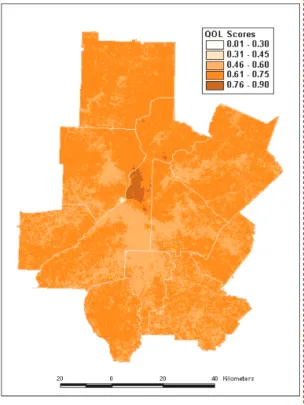
FIGURE 5. Urban quality of life scores, 2000 methodological difficulties associated with
the WLC and AHP methods (Carver, 1991;
Can, 1992; Malczewski, 2006). In the CDA method, each pair of alternatives is analyzed for the degree to which one out‐ranks the other on the specified criteria. The CDA method is computationally impractical when a large number of alternatives are present (Eastman et al., 1995; Malczewski, 1999;
Malczewski, 2006). In case of raster data, every pixel is an alternative. However, the WLC method is very straightforward in a raster GIS environment. In this regard, the SMA approach based on the WLC method was implemented to integrate and transform eight variables into a resultant QOL score for each pixel. The weighted standardized criteria were then aggregated to generate the overall QOL score using a decision rule based on the WLC method. This operation was achieved by the GIS overlay (add) function in ArcView GIS. Because the weights sum to 1 and the criteria were standardized from 0 to 1, the resultant QOL score ranges from 0 to 1. The best QOL score is 1 while the worst is 0.
FIGURE 5 shows the overall QOL score map generated by the SMA approach based on the WLC method in conjunction with the linear scale transformation method for standardizing the criteria and the AHP method for deriving the criterion weights.
The QOL score ranging from 0.01 to 0.90 was obtained in this study. The highest QOL score was found around Buckhead, Sandy Springs, Riverside, Roswell, and Alphretta whereas the lowest QOL score was found around Smyrna in Cobb County.
The major urbanized areas and the southern
central city of Atlanta showed relatively lower QOL scores than their counterparts.
The extent of spatial clustering of QOL scores was examined by Moran’s I.
According to the statistics, the spatial autocorrelation coefficient was 0.99 for only pixels covering the Atlanta metropolitan area. This confirms that there existed a strong spatial polarization of the QOL scores in the Atlanta metropolitan area. Therefore, it is suggested that sustainable urban development policies are required to control the location of industrial facilities, urban land use, vegetation cover, and transportation in the Atlanta metropolitan area.
According to the visual map comparison between FIGURE 5 and the QOL score map generated by the PCA approach in the previous study (Jun, 2006b), it is found that
the spatial patterns were slightly different at the global scale. In order to verify the spatial similarity, a correlation analysis between the QOL score map based on the SMA approach and the QOL score map based on the PCA approach was performed in ERDAS Imagine. The resulted correlation coefficient was 0.99 and the coefficient of determination was 0.98 for only pixels covering the Atlanta metropolitan area. The two maps are spatially strongly correlated with each other. This implies that the performance of the SMA approach to urban QOL assessment proves comparable to that of the PCA approach, which is an objective approach to urban QOL assessment.
2. Implications for Future Research There are several methodological issues to be taken into consideration for the pixel‐
based SMA approach to urban QOL assessment. First, it would be desirable to conduct a sensitivity analysis in order to test the variability of the resultant QOL scores to changes in the decision maker’s preferences. Urban QOL assessment often involves multiple solutions and several different approaches to reach these solutions.
The consequences of using different criteria weights may lead to different QOL scores.
The robustness of the QOL model generated in this study needs to be evaluated by a sensitivity analysis (Malczewski, 1999).
Second, urban QOL needs to be evaluated by a number of decision makers. The SMA approach developed in this study supports a subjective expert‐based spatial decision making for urban QOL evaluation. However, the urban QOL evaluation is typically
complex in nature and the decision makers are characterized by different preference structures with respect to the relative importance of criteria on the basis of the urban QOL evaluation (Rinner, 2007). It is necessary to extend the SMA approach for group and participatory decision making (Malczewski, 2006).
Third, the urban QOL assessment possesses uncertainty about the concepts, rules, and principles involved to reach multiple solutions. The literature review indicates that there are a number of contrasting definitions of what QOL means as well as there is no consensus on the selection of QOL indicators. In addition, there are several conflicting approaches on the processing of QOL indicators. Fuzzy logic can be used to deal with uncertainty associated with imprecision concerning the urban QOL assessment (Banai, 1993;
Malczewski, 1999; Rashed and Weeks, 2003;
Malczewski, 2006).
CONCLUSION
In this research, a SMA approach was demonstrated to evaluate urban QOL in a raster GIS environment. Three methods were involved to implement the SMA approach to urban QOL assessment. First, the linear scale transformation method was used to standardize eight variables such as three environmental variables (urban use, NDVI, and surface temperature), a hazard‐
related variable (cumulative potential relative exposure values to TRI facilities), and four socioeconomic variables (population density, percent college graduates, per capita income,
and median home values) at different measurement scales. This method contributed to operationally dealing with inappropriate scaling of several incommensurate criteria. Second, the AHP method was employed to structure the multicriteria evaluation of urban QOL and to assign the weights of relative importance to the eight criteria. The AHP method would be computationally practical for a pairwise comparison of a large number of alternatives in a raster GIS environment since this method assisted in simplifying the spatial decision problem by creating a hierarchy of criteria. The AHP method also allowed for effectively eliciting the decision maker’s preferences to multiple criteria so that it could treat much unstructured subjectivity in the decision maker’s judgment. Third, the WLC method was used to aggregate the criteria and their relative weights in additive fashion. The WLC method was easy to implement in a raster GIS environment using map algebra operations and cartographic modeling. In this manner, the SMA approach developed in this study helped with conducting the multicriteria evaluation of urban QOL in a raster GIS environment.
The SMA approach was implemented with a case study of the urban QOL evaluation in the Atlanta metropolitan area in 2000. The resultant QOL score map was visually and statistically compared with the QOL score map generated by the PCA approach in the previous study (Jun, 2006b) to evaluate its performance. The visual and statistical results indicate that the two QOL score maps are spatially strongly correlated
with each other. In other words, the results prove that the SMA approach to urban QOL assessment, a subjective approach, would be comparable to the PCA approach which is an objective approach. This implies that the SMA approach proposed in this research may provide an alternative approach for analyzing the QOL in an urban environment.
In the near future, the proposed methodology awaits potential contributions from the field of geocomputation.
ACKNOWLEDGEMENT
This research was supported by Kyungpook National University Research Fund, 2007.
REFERENCES
Apparicio, P., A.‐M. Seguin and D. Naud.
2008. The quality of the urban environment around public housing buildings in Montreal:
an objective approach based on GIS and multivariate statistical analysis. Social Indicators Research 86(3):355-380.
Banai, R. 1993. Fuzziness in geographical information systems: contributions from the analytical hierarchy process. International Journal of Geographical Information Systems 7(4):315-329.
Bederman, S.H. and T.A. Hartshorn. 1984.
Quality of life in Georgia: the 1980 experience. Southeastern Geographer 24(2):78-98.
Can, A. 1992. Residential quality assessment:
alternative approaches using GIS. The Annals of Regional Science 26:97-110.
Carver, S. 1991. Integrating multi‐criteria evaluations with geographical information systems. International Journal of Geographical Information Systems 5(3):321-339.