환경적 형평성과 도시 삶의 질의 공간적 관계에 대한 탐색
전병운1※
Exploring the Spatial Relationships between Environmental Equity and Urban Quality of Life
Byong‐Woon JUN1※
1
ABSTRACT
Although ordinary least squares (OLS) regression analysis can be used to examine the spatial relationships between environmental equity and urban quality of life, this global method may mask the local variations in the relationships between them. These geographical variations can not be captured without using local methods. In this context, this paper explores the spatially varying relationships between environmental equity and urban quality of life across the Atlanta metropolitan area by geographically weighted regression (GWR), a local method. Environmental equity and urban quality of life were quantified with an integrated approach of GIS and remote sensing. Results show that generally, there is a negatively significant relationship between them over the Atlanta metropolitan area. The results also suggest that the relationships between environmental equity and urban quality of life vary significantly over space and the GWR (local) model is a significant improvement on the OLS (global) model for the Atlanta metropolitan area.
KEYWORDS : GWR, Environmental Equity, Quality of Life, Spatial Non‐Stationarity
요 약
OLS 회귀분석은 환경적 형평성과 도시 삶의 질의 공간적 관계를 밝히기 위하여 사용되어 질 수 있지만, 이러한 전역적 방법은 그 공간적 관계에 있어서 국지적 변이를 설명할 수 없다. 이들 지리적 변이를 밝혀 내기 위해서는 반드시 국지적 방법을 사용해야 한다. 이러한 맥락에서, 본 논 문은 국지적 방법인 지리적 가중회귀분석(GWR)을 이용하여 애틀란타 대도시권에서 환경적 형평 성과 도시 삶의 질간의 공간적 변이관계를 탐색하고자 한다. 환경적 형평성과 도시 삶의 질은
2011년 8월 10일 접수 Received on August 10, 2011 / 2011년 9월 10일 수정 Revised on September 10, 2011 / 2011년 9월 20일 심사완료 Accepted on September 20, 2011
1 경북대학교 지리학과 Department of Geography, Kyungpook National University
※ 연락저자 E‐mail : [email protected]
GIS와 원격탐사의 통합적 방법에 의하여 측정되었다. 연구결과에 따르면, 애틀란타 대도시권에서 환경적 형평성과 도시 삶의 질의 공간적 관계는 일반적으로 유의적인 부의 관계가 있었다. 또한, 환경적 형평성과 도시 삶의 질의 관계는 공간상에서 상당히 변이하고, 전역적 OLS 모델 보다 GWR 모델이 이러한 공간적 변이관계를 더 잘 설명할 수 있는 것으로 나타났다.
주요어 : 지리적 가중회귀분석, 환경적 형평성, 삶의 질, 공간적 이질성
INTRODUCTION
Environmental justice is the principle that all people should bear a proportionate share of environmental costs such as pollution and health risk and rejoice at equal access to environmental amenities (Harner et al., 2002). A fundamental question in environmental justice analysis concerns environmental equity that investigates if the spatial distribution of environmental risks and amenities is equitable among diverse racial and socioeconomic groups.
In the U.S.A., environmental justice policies have tried to create environmental equity within the society since early 1990. Research concerns for environmental equity have been mainly focused on human health effects from environmental hazards. Recently, attention has also been given to multiple dimensions of impacts from environmental hazards such as environmental, social, and economic impacts, in addition to health risk (Liu, 2001).
Research focus for urban environmental equity has been largely confined to potential exposure to toxic sites, but the research focus has recently expanded to certain other environmentally sensitive issues such as a zone of urban blight, open space, parks, transportation
systems, and urban sprawl (Liu, 2001;
Harner, et al., 2002). Liu (2001) suggested that it is necessary to incorporate major environment risks and amenities for urban environmental equity analysis. Further, Holifield (2001) pointed out the need to broaden the usual conception of environment in order to open new possibilities in environmental equity research. Therefore, it is apparent that the final goal of urban environmental equity analysis needs to be extended to evaluate the quality of life (QOL) of people in the community. Although QOL has not been expressed adequately so far, it is related to the general well-being of people (Jun, 2008).
Investigating the relationships between environmental equity and QOL in urban regions is important for two reasons.
First, it is required to examine the role of environmental risks in the spatial variation of QOL. Second, this can help urban planners and decision‐makers to be aware of any problem areas in the allocation of urban services. It is particularly true in areas where there is concern about building sustainable growth management plans. However, little attention is given to this topic in the urban environmental equity and QOL research community.
Ordinary least squares (OLS) regression analysis can be employed to
disentangle the interrelationships between environmental equity and QOL. OLS regression models of spatial data may show spatial non‐stationarity referring to the fact that the relationships among independent and dependent variables are different across space (Fotheringham et al., 1996). This global method may mask the local variations in the relationships between them. These geographical variations can not be captured without using local methods. In this regard, this research explores the spatially varying relationships between environmental equity and QOL across the Atlanta metropolitan area using geographically weighted regression (GWR), a local method. After a brief introduction, an overview of GWR is described. Data and methods are then presented and followed by the introducing of the results with a discussion of them. The last section contains summary and concluding remarks.
GWR AND SPATIAL NON‐STATIONARITY
GWR is an exploratory spatial data analysis (ESDA) technique that can be used to investigate the nature of spatial non‐stationarity in OLS regression models of spatial data. GWR builds on a global regression model expressed as:
i k
ik k
i x
y =a0 +åa +e (1)
GWR extends this global regression model by allowing the local estimation of
model parameters at each observation’s location (Fotheringham et al., 2002). The equation may thus be revised as follows:
i k
ik i i k i
i
i u v u v x
y =a0( , )+åa ( , ) +e (2)
where (ui, vi) indicates the coordinates of the location of observation i. Specifically, GWR is calibrated by weighting all neighboring observations on the basis of a distance decay function away from observation i. GWR then generates a set of local regression results including local parameter estimates, the values of t‐test on the local parameter estimates, the local R2 values, and the local residuals for each regression point. Finally, the local model parameters can be mapped using geographic information system (GIS) software so that local variations in the regression results can be detected.
Therefore, GWR provides a useful tool to explore the spatially varying relationships between environmental equity and QOL.
In recent years, GWR has been increasingly applied in various fields such as ecology, land use studies, social studies, and environmental studies to explore the spatially varying relationships. Longley and Tobon (2004) explored spatial dependence and heterogeneity in the determinants of deprivation in Bristol, U.K. Mennis and Jordan (2005) revealed the relationships among race, class, employment, urban concentration, and land use with air toxic release density in New Jersey, USA.
Clement et al. (2009) identified drivers of forest transition in a province of
Northern Vietnam between 1993 and 2000. Ogneva‐Himmelberger et al. (2009) explored regional variations in the relationship between socio‐economic variables and green vegetation land cover across the state of Massachusetts, USA.
Harris et al. (2010) quantified spatial relationships between freshwater acidification critical load data and contextual catchment data across Great Britain and calibrated robust GWR unlike many previous studies. Lloyd (2010) demonstrated how GWR statistics can be used to explore the degree to which single socioeconomic and demographic variables and relations between such variables differ at different scales and at different geographic locations in Northern Ireland. Scull (2010) investigated the relationship between climate and soil character across the contiguous United States. Gao and Liu (2011) detected location‐dependent and scale‐dependent relationships between urban landscape fragmentation and related factors in Shenzhen City, Guangdong Province, China. Tu (2011) found significant relationships between land use and water quality across watersheds in eastern Massachusetts, USA. However, there is no research that assesses the application of GWR for exploring the spatially varying relationships between environmental equity and QOL at any scale of analysis.
DATA AND METHODS
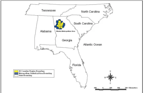
This research chose the Atlanta metropolitan area in the Southeastern U.S. as a case study area (FIGURE 1).
This study area comprises 10 metro
counties. There have been some controversial environmental and QOL issues in the study area such as urban heat island effect detected, degenerated air quality, water‐quality issues related to urban development, and paradoxical urban landscape based on racial segregation (Sjoquist, 2000). In this study area, there thus existed a need to explore the spatially varying relationships between environmental equity and QOL.
The QOL in the Atlanta metropolitan area, 2000 was quantified in terms of demographic, economic, educational, housing, environmental, and hazard‐related factors by the integrated approach of GIS and remote sensing developed in the previous study (Jun, 2006b). Four socioeconomic variables (such as population density, per capita income, percent college graduates, and median home value) derived from census data in 2000 are zonal data whereas three environmental variables (such as land use and cover, normalized difference vegetation index (NDVI), and surface temperatures) extracted from Landsat TM 5 data in 2000 and a hazard‐related variable (such as cumulative potential relative exposure to toxic release inventory (TRI) facilities extracted from the TRI database in 2000) are per‐pixel data. The environmental and hazard‐
related variables were spatially aggregated into census block groups to integrate two different areal units of data and to perform further analysis. A principal components analysis (PCA) approach was then used to transform environmental, hazard‐related, and socioeconomic variables into a resultant
FIGURE 1. Location of study area
QOL score for each census block group.
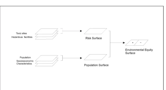
To determine the environmental equity, an environmental equity model was developed in this research by identifying the spatial clustering of hot spots in environmental equity as illustrated in FIGURE 2. This model provides us with the spatial variations in environmental equity within a defined urban region. By combining a risk surface and a population surface, the environmental equity model was performed. The risk surface was generated using the equation proposed by Cutter et al. (2001). In specific, the cumulative proximal exposure (CPE) to population in each census unit from distance to TRI facilities was calculated and then weighted by the relative potential risk score (RPRS) for a given
TRI facility to utilize the magnitude and the relative toxicity of release from TRI facilities. The population surface for percentages of minority and people below poverty level was constructed using the methodology in the previous study (Jun, 2006a). The weighted linear combination method in GIS environment was employed to integrate two surfaces and then to create an environmental inequity surface in the Atlanta metropolitan area, 2000. The environmental inequity scores were spatially aggregated into census block groups for further analysis.
The resultant QOL score map was visually and statistically compared with the environmental inequity score map for 2000 in order to investigate the spatially varying relationships between them. For
FIGURE 2. An approach to modeling environmental equity in a GIS context statistical investigation, OLS regression
and GWR were performed for a pair of maps, respectively. OLS regression is called a global method because this method produces a global predictive model. However, GWR is called a local method since this method expresses the spatial variation in model parameter estimates. Following the OLS regression, GWR and choropleth mapping were implemented to explore spatial non‐
stationarity.
The GWR 2.2 software package for GWR analysis was used in this study. In calibrating a GWR model, the geographical weighting scheme needs to be specified.
To do so, the specification of a kernel shape and a bandwidth is required (Fotheringham et al., 2002). In this study, an adaptive kernel was chosen because this kind of kernel permits use of a variable bandwidth. If the distance between the regression point and the data point is greater than the bandwidth,
the weight of the data point is zero.
Otherwise, the weight of the data point is calculated using a bi‐square function. In this study, the optimal bandwidth was determined by using all the data entered and then selecting the bandwidth that minimizes the Akaike Information Criterion (AIC). The Golden Section search technique was applied to minimize the AIC. Finally, a Monte Carlo significance test was used to determine whether any of the local parameter estimates are significantly nonstationary so that we can consider whether the local model offers an improvement over the global model.
RESULTS AND DISCUSSION
The spatial relationships between environmental equity and QOL were explored by visual and statistical analyses. In order to investigate the spatial relationships between them, the
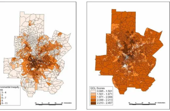
FIGURE 3. Environmental inequity surface, 2000
FIGURE 4. Urban QOL scores, 2000 QOL score map was visually compared
with the environmental inequity score map for 2000. The visual comparison between FIGURE 3 and FIGURE 4 revealed that the overall spatial pattern was inversed in the Atlanta metropolitan area. In other words, the areas (around the southern central city of Atlanta, Tri‐
cities, Norcross, Marietta/Smyrna, Conyer, and midtown) with higher environmental inequity scores appeared around those (around downtown Atlanta, Smyrna, and Hartsfield‐Jackson international airport) with lower QOL scores while the places (around the northern parts of Fulton County along Georgia 400, the northern central city of Atlanta, and many suburbs) with lower environmental inequity scores occurred around those (around Sandy Spring, Roswell,
Alpharetta, and the northern parts of Fulton County along Georgia 400) with higher QOL scores.
The reverse spatial relationships between environmental equity and QOL were statistically verified. This was achieved by performing OLS regression and GWR analysis of the environmental inequity score map against the QOL score map in the Atlanta metropolitan area. The results from the OLS regression analysis indicate that the correlation coefficient between the environmental inequity score map and the QOL score map was ‐0.39 or a coefficient of determination of 15 percent. However, the results from the GWR analysis show that the correlation coefficient between them was ‐0.87 or a coefficient of determination of 75
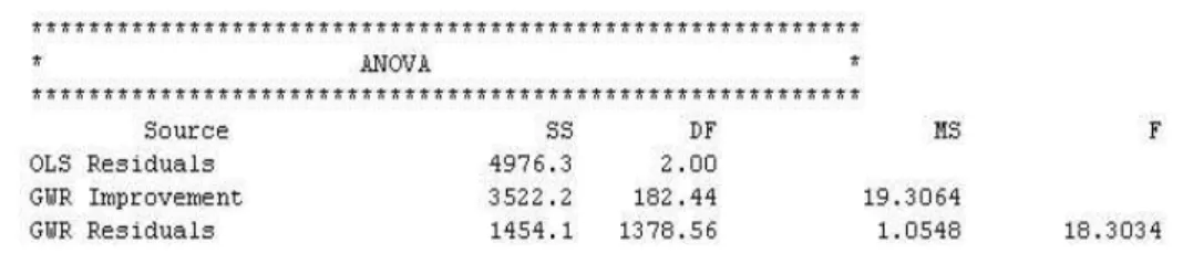
FIGURE 5. ANOVA results
FIGURE 6. Results of Monte Carlo test for spatial non‐stationarity
percent. This indicates that there were globally not significant relationships between environmental equity and QOL in the study area, but there were locally some significant relationships between them. The result from the ANOVA test as shown in FIGURE 5 suggests the fact that the GWR (local) model is a significant improvement on the OLS (global) model in explaining the spatial relationships between them in the Atlanta metropolitan area. The statistical results thus confirmed that the environmental inequity scores are significantly negatively correlated with the QOL scores in the Atlanta metropolitan area in 2000.
The visual and statistical analyses
showed that the spatial relationships between environmental equity and QOL vary significantly over space. The Montel Carlo significance test for spatial variability of local parameters as shown in FIGURE 6 demonstrates that conventional OLS regression conceals important local variations in the relationships between environmental equity and QOL. In other words, this spatial non‐stationarity is significant within the Atlanta metropolitan area.
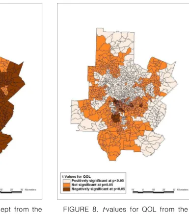
GWR, in combination with choropleth mapping, divulges the nature of spatial non‐stationarity in the spatial relationships between environmental equity and QOL in the Atlanta metropolitan area. FIGUREs 7 and 8 show t‐values for intercept and
FIGURE 7. t‐values for intercept from the GWR model of environmental equity and
QOL
FIGURE 8. t‐values for QOL from the GWR model of environmental equity and
QOL QOL from the GWR model of
environmental equity and QOL. Note that maps of the intercept and QOL show positively and negatively significant t‐
values (p<0.05) in light orange and dark orange, respectively. The medium orange indicates areas that are not significant.
The intercept is negatively significant over a large area covering the northern parts of Fulton County along Georgia 400, downtown Atlanta, the southwestern suburbs, and the southeastern suburbs.
This indicates that these areas have reduced the environmental inequity scores even after the variation in QOL has been accounted for. The QOL is positively significant around the northern
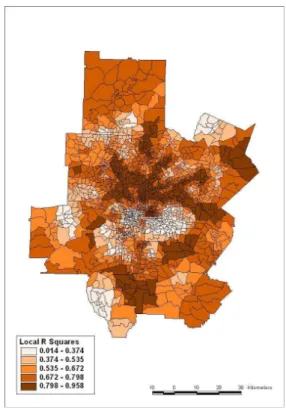
parts of Fulton County along Georgia 400 and some portions of the southwestern and southeastern suburbs. This suggests that higher environmental inequity scores are related to higher QOL scores. In contrast, significant negative relationships are found in some portions of the southern central city of Atlanta. This indicates that higher environmental inequity scores are associated with lower QOL scores. FIGURE 9 shows local R2 values for the GWR model of environmental equity and QOL. The ability of QOL to explain the spatial variations in the environmental inequity scores also changes across the study area because the local R2 values show
FIGURE 9. Local R2 values for the GWR model of environmental equity and QOL considerable differences. High values are
mainly observed around the northern parts of Fulton County along Georgia 400, where QOL can explain 80~96% of the variances in the environmental inequity scores, while low values are distributed around the southern central city of Atlanta, where it only captures 1‐
37% of the variances. The spatial variations in significance and local R2 for the relationships between environmental equity and QOL confirm that significant spatial non‐stationarity exists in the relationships between them in the Atlanta metropolitan area. Thus, GWR is a more appropriate method than traditional OLS regression analysis in the study area.
This research brings up some
theoretical and methodological issues to be taken into consideration. First, this study has implications for environmental equity analysis and urban QOL assessment. It is clearly noted that at least in the study area, urban QOL assessment can complement environmental equity analysis because environmental equity can be predicted by QOL with the help of GWR and the QOL assessment can provide a more comprehensive perspective for investigating urban environmental equity issues. Second, there is a methodological issue related to calibrating robust GWR models. The GWR model developed in this study employed all the data entered (e.g. 1563). All the data may be filtered to screen out
outlying observations so that a more robust GWR model can be calibrated (Harris et al., 2010). Third, this research is still subjected to the modifiable areal unit problem (MAUP). In this study, the data aggregation unit is census block group. If the spatial unit changes to census tract, the analytical results of GWR may be different. In future research, this topic needs to be thoroughly explored. Fourth, it is necessary to develop a standard approach for improving mapping of the results of GWR (Mennis, 2006). The cartographic approach used in this study may ineffectively depict the spatial distribution of the sign, magnitude, and significance of the influence of each independent variable on the dependent variable. Thus, a new approach is required to facilitate exploring spatial non-stationarity.
CONCLUSION
The spatially varying relationships between environmental equity and QOL were investigated by statistical analyses such as OLS regression and GWR. It was found that generally, there was a negatively significant relationship between environmental equity and QOL across the Atlanta metropolitan area. However, the statistical results indicated that the spatial relationships between environmental equity and QOL vary significantly over space. The results also suggested that the GWR (local) model is a significant improvement on the OLS (global) model in explaining the spatial relationships between environmental equity and QOL in
the Atlanta metropolitan area. Further research in other cities is required to investigate the nature of spatial non‐
stationarity in the spatial relationships between environmental equity and QOL.
This research demonstrates that the integrated approaches of GIS and remote sensing, in combination with GWR, can provide a useful tool for policy makers, regional and local agencies, and researchers to unveil urban structure and to test urban theories.
ACKNOWLEDGEMENTS
This research was supported by Kyungpook National University Research Fund, 2008.
REFERENCES
Clement, F., D. Orange, M. Williams, C.
Mulley and M. Epprecht. 2009. Drivers of afforestation in Northern Vietnam:
assessing local variations using geographically weighted regression.
Applied Geography 29:561‐576.
Cutter, S.L., M.E. Hodgson and K. Dow.
2001. Subsidized inequities: the spatial patterning of environmental risks and federally assisted housing. Urban Geography 22(1):29‐53.
Fotheringham, S.A., C.F. Brunsdon and M.E. Charlton. 2002. Geographically Weighted Regression: The Analysis of Spatially Varying Relationships.
Chichester, U.K.: Wiley. 269pp.
Fotheringham, S.A., M.E. Charlton and C.F. Brunsdon. 1996. The geography of
parameter space: an investigation into spatial nonstationarity. International Journal of Geographical Information Systems 10:605‐627.
Gao, J. and S. Li. 2011. Detecting spatially non‐stationary and scale‐
dependent relationships between urban landscape fragmentation and related factors using geographically weighted regression. Applied Geography 31:292‐
302.
Harner, J., K. Warner, J. Pierce and T.
Huber. 2002. Urban environmental justice indices. The Professional Geographer 54(3):318‐331.
Harris, P., A.S. Fortheringham and S.
Juggins. 2010. Robust geographically weighted regression: a technique for quantifying spatial relationships between freshwater acidification critical loads and catchment attributes. Annals of the Associations of American Geographers 100(2):286‐306.
Holifield, R. 2001. Defining environmental justice and environmental racism. Urban Geography 22(1):78‐90.
Jun, B.W. 2006a. An evaluation of a dasymetric surface model for spatial disaggregation of zonal population data.
Journal of The Korean Association of Regional Geographers 12(5):614‐630.
Jun, B.W. 2006b. Urban quality of life assessment using satellite image and socioeconomic data in GIS. Korean Journal of Remote Sensing 22(5):325‐
335.
Jun, B.W. 2008. A spatial multicriteria analysis approach to urban quality of
life assessment. Journal of The Korean Association of Geographic Information Studies 11(4):122‐138.
Liu, F. 2001. Environmental Justice Analysis: Theories, Methods, and Practice. New York, NY: Lewis Publishers. 367pp.
Lloyd, C.D. 2010. Exploring population spatial concentrations in Northern Island by community background and other characteristics: an application of geographically weighted regression.
International Journal of Geographical Information Science 24(8):1193‐1221.
Longley, P.A. and C. Tobon. 2004. Spatial dependence and heterogeneity in patterns of hardship: an intra‐urban analysis. Annals of the Associations of American Geographers 94(3):503‐519.
Mennis, J. 2006. Mapping the results of geographically weighted regression. The Cartographic Journal 43(2):171‐179.
Mennis, J. and L. Jordan. 2005. The distribution of environmental equity:
exploring spatial nonstationarity in multivariate models of air toxic releases. Annals of the Association of American Geographers 95(2):249‐268.
Ogneva‐Himmelberger, Y., H. Pearsall and R. Rakshit. 2009. Concrete evidence and geographically weighted regression:
a regional analysis of wealth and the land cover in Massachusetts. Applied Geography 29:478‐487.
Scull, P. 2010. A top‐down approach to the state factor paradigm for use in macroscale soil analysis. Annals of the Associations of American Geographers
100(1):1‐12.
Sjoquist, D.L.(ed.). 2000. The Atlanta Paradox. New York, NY: Russell Sage Foundation. 300pp.
Tu, J. 2011. Spatially varying
relationships between land use and water quality across an urbanization gradient explored by geographically weighted regression. Applied Geography 31:376‐392.