도시의 삶의 질을 평가하기 위한 화소기반 기법
전병운1※
A Pixel‐based Assessment of Urban Quality of Life
Byong‐Woon JUN1※1
요 약
소수의 선행연구는 도시의 삶의 질을 평가하기 위해서 구역을 단위로 사회경제적인 자료와 원격 탐사자료를 통합하려고 시도했다. 그러나 이러한 구역을 기반으로 한 접근방법은 한 단위구역의 모 든 속성이 그 구역 내에서 균등하게 분포되어 있다고 비현실적으로 전제할 뿐만 아니라, 임의적 지 역구획문제 (MAUP) 및 화소기반 환경자료와의 통합이 용이하지 않은 점과 같은 심각한 방법론적 어려움을 초래한다. 구역기반 접근방법에 대한 한 가지 대안은 기본적인 공간단위로서 화소를 이용 하는 화소기반 접근방법이다. 본 연구에서는 도시의 삶의 질을 평가하기 위해서 GIS에서의 사회경 제적인 자료와 원격탐사자료를 연계하기 위한 화소기반 접근방법을 제시하고자 한다. 화소기반 접 근방법은 삶의 질을 평가하기 위해서 구역기반의 사회경제적인 자료를 개별 화소들로 더욱 세분화 시키려고 밀도 구분도와 공간 내삽법의 원리를 이용하고, 그 세분화된 사회경제적인 자료와 원격탐 사자료를 통합한다. 이러한 화소기반 접근방법은 조지아 풀톤 카운티에 대한 사례연구에서 적용되 었고, 같은 사례지역에서의 구역기반 접근방법과도 비교되었다. 본 연구에서 도시의 삶의 질을 평가 하기 위한 화소기반 접근방법은 구역단위의 사회경제적인 자료의 세분화를 위해서 많은 처리시간을 필요로 하지만, 미시적인 지표의 산출을 용이하게 하고 사회경제적인 자료와 원격탐사자료간의 효 율적인 통합과 그러한 자료들의 시각화를 가능하게 하였다. 이러한 점에서, 본 연구는 화소기반 접 근방법이 도시 분석에 있어서 새로운 데이터베이스의 구축과 분석능력의 향상에 기여할 수 있다는 가능성을 제시한다.
주요어 : 지리정보시스템, 위성영상, 밀도 구분적 지도화, 공간 내삽법, 도시 삶의 질
ABSTRACT
A handful of previous studies have attempted to integrate socioeconomic data and remotely sensed data for urban quality of life assessment with their spatial dimension in a zonal unit.
However, such a zone-based approach not only has the unrealistic assumption that all attributes of a zone are uniformly spatially distributed throughout the zone, but also has resulted in serious methodological difficulties such as the modifiable areal unit problem and the
2006년 7월 13일 접수 Received on July 13, 2006 / 2006년 9월 11일 심사완료 Accepted on September 11, 2006 1 미국 루이지애나공대 사회과학학과 Department of Social Sciences, Louisiana Tech University, USA
※ 연락저자 E-mail : [email protected]
incompatibility problem with environmental data. An alternative to the zone-based approach can be a pixel-based approach which gets its spatial dimension through a pixel. This paper proposes a pixel-based approach to linking remotely sensed data with socioeconomic data in GIS for urban quality of life assessment. The pixel-based approach uses dasymetric mapping and spatial interpolation to spatially disaggregate socioeconomic data and integrates remotely sensed data with spatially disaggregated socioeconomic data for the quality of life assessment.
This approach was implemented and compared with a zone-based approach using a case study of Fulton County, Georgia. Results indicate that the pixel-based approach allows for the calculation of a microscale indicator in the urban quality of life assessment and facilitates efficient data integration and visualization in the assessment although it costs an intermediate step with more processing time such as the disaggregation of zonal data. The results also demonstrate that the pixel-based approach opens up the potential for the development of new database and increased analytical capabilities in urban analysis.
KEYWORDS : GIS, Satellite Image, Dasymetric Mapping, Spatial Interpolation, Urban Quality of Life
INTRODUCTION
Although the integrated use of remotely sensed data and GIS-based data has been explosively made for environmental applications, the integration for socioeconomic applications has received relatively less attention and has been rapidly developing in recent years (Martin and Bracken, 1993;
Martin, 1996; Mesev, 2003). Several attempts have been made to integrate remotely sensed data with socioeconomic data in geographic information systems (GIS). One of the major socioeconomic applications is related to quality of life assessment. A handful of previous studies (Forster, 1983; Weber and Hirsh, 1992; Lo and Faber, 1997) have assessed quality of life indicators in urban areas by integrating biophysical variables derived from satellite images and socioeconomic variables extracted from census data. These studies demonstrated that such an integration provides a more detailed characterization of urban landscape than an
approach based solely on socioeconomic data.
Despite their benefit, there is a fundamental technical problem, namely differences in areal units (Chen, 2002), inherent in the previous studies on urban quality of life assessment. Socioeconomic data are zonal data (e.g., census zones or administrative boundaries) while environmental data derived from remotely sensed images are per-pixel data (e.g., 30 m for Landsat TM images). Conceptually, these two areal units are not compatible. For their economical operation and computational feasibility, previous studies have aggregated pixel-based data to zonal units to tackle the incompatibility problem in areal units.
However, the zone-based approach unrealistically assumes that all the socioeconomic data are uniformly distributed within zonal units and ignores the fact that socioeconomic activities and their impacts are continuous in space. This approach also has analytical pitfalls such as the modifiable areal unit problem (MAUP) and the
incompatibility problem with environmental data. Moreover, most urban analyses have become increasingly disaggregated in space, time, and substantive elements (Spiekermann and Wegener, 2000). As an alternative to the zone-based approach, a pixel-based approach can be used to spatially disaggregate socioeconomic data within an enumeration unit such as a census tract and a census block group into individual pixels. This topic has not been thoroughly studied in the GIS and remote sensing research community.
In this context, this paper proposes a pixel-based approach to integrating remotely sensed data and socioeconomic data in GIS for the quality of life assessment in an urban area. After a brief introduction, an overview of quality of life research is presented. The methodology is then introduced and followed by the results with a discussion of them. The last section contains concluding remarks and summary.
QUALITY OF LIFE RESEARCH
The quality of life of a population is an important concern in social sciences, but it has no consensus definition. According to sociologists, quality of life is a collective trait pertaining to groups of people, not to individuals. Various indicators consisting of both objective and subjective elements can be used to quantify it (Bederman and Hartshorn, 1984). Even though there is no single definition and no broadly accepted method to measure quality of life, it appears clear from the literature that some consensual objective indicators such as income, housing, education and crowding have been widely used to measure quality of
life (Wallace, 1971; Smith, 1973; Liu, 1976).
The majority of previous quality of life evaluation studies utilized only socioeconomic indicators from census data as exemplified by the works of Liu (1976) and Bederman and Hartshorn (1984).
Recent advances in satellite remote sensing and GIS technologies have helped to streamline the integration of socioeconomic data with remotely sensed data for urban studies (Mesev, 2003). With the increasing concern about environmental issues, biophysical data derived from remotely sensed images have been employed for quality of life assessment. Forster (1983) developed a residential quality index in the city of Sydney, Australia, using spectral reflectance values derived from Landsat MSS images. He employed house size and vegetation content as a positive indicator of quality and roads and nonresidential buildings as a negative indicator. Weber and Hirsch (1992) measured the urban life quality of Strasbourg, France, by combining the high-resolution SPOT XS image data with cartographic and census data. Most recently, Lo and Faber (1997) demonstrated the usefulness of Landsat TM image in conjunction with census data for quality of life assessment in a small city in Georgia with emphasis on NDVI as a desirable quality indicator of urban morphological environment. Lo and Faber argued that satellite image data could complement census data in providing an environmental perspective for the quality of life assessment.
Therefore, the inclusion of environmental data has allowed for taking a more complete picture of the quality of life by relating environmental quality to social quality (Lo
and Faber, 1997). Based on the literature review, it is apparent that within the GIS and remote sensing research community, urban quality of life was measured with the use of scales or indices which coupled the socioeconomic with environmental data for a complete evaluation. The quality of life assessment can help urban planners and city decision-makers to find out any problem areas in the allocation of human services.
DATA AND METHODS
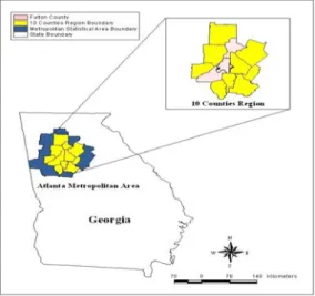
In this study, Fulton County, Georgia serves as a case study area where the core city of Atlanta is located as shown in Figure 1. The study area was chosen because of its urban heat island effect detected, degenerated air quality, water quality issues related to urban development downstream of the upper Chattahoochee River, and high levels of urban inequality based on racial segregation. The study area thus provides a unique urban setting for a quality of life assessment.
FIGURE 1. Location of study area
Figure 2 illustrates an overview of the research methodology implemented for this study. The quality of life in the study area was evaluated and mapped on the basis of demographic, economic, educational, housing, and environmental factors. Most of the criteria for
quality of life assessment were selected as suggested by Lo and Faber (1997). Two major data sources include demographic and socioeconomic data from 1990 Census and environmental data from 1990 Landsat 5 TM imagery.
FIGURE 2. Research methodology
From the Landsat TM image, derived were three environmental data such as land use and cover, normalized difference vegetation index (NDVI), and surface temperature. A land use and cover map was extracted from the Landsat TM image using a hybrid digital image classification and a modified version of the Anderson scheme of
land use and cover classification with mixed levels 1 and 2. From this land use and cover map, the low density residential, high density residential, commercial and industrial (urban use), forest, and agriculture (comprising grassland/pasture/cropland) classes were extracted and water and barren classes were excluded using a reclassification method. The overall accuracy of the land use and cover map was determined to be 87.5 percent. The classification accuracy is good enough to meet the minimum 85 percent accuracy requirement recommended by the Anderson classification scheme (Anderson et al., 1976) and thus is sufficient for further applications.
From bands 3 and 4 of the Landsat TM image, NDVI was computed for each pixel using the following equation:
3 4
3 4
TM TM
TM NDVI TM
+
= −
(1)
where TM3 is band 3 of Landsat TM image and TM4 is band 4 of the image. The index varies from –1 to +1 as greenness increases. From the thermal infrared band, band 6 of the Landsat TM image, surface temperature for each pixel was also computed using the following equation proposed by Wukelic et al. (1989):
L ) (K K K T
1 1 ln ) 2 (
+
=
(2)
where T(K) is effective at-satellite temperature in Kelvin, K2 is calibration constant 2 (=1260.56) in Kelvin, K1 is calibration constant 1 (=607.76) in w.m-2.ster-1.mm-1, and L is spectral radiance in w.m-2.ster-1.mm-1.
Basically, this equation converts the spectral radiances of image pixels into at-satellite temperatures. The resultant at-satellite temperatures were then corrected for emissivity (ε) according to the nature of land cover. In general, vegetated areas are given a value of 0.95 and non-vegetated areas 0.92 (Nichol, 1994). This differentiation is based on the NDVI image calculated as described above. The emissivity corrected surface temperature (Ts) is computed as follows (Nichol, 1994):
ε ) T(K)/
( T
sT(K)
ln
1 + λ α
=
(3)where λ is the wavelength of emitted radiance (= 11.5 μm), α is hc/k (1.438 * 10-2 mK), k is Stefan-Bolzmann’s Constant (1.38
* 10-23 J/K), h is Planck’s constant (6.26 * 10-34 J-sec), c is velocity of light (2.998 * 108 m/sec), and ε is surface emissivity.
These absolute temperatures were then converted into Celsius (C) by subtracting the temperature of the ice point (273.15 K) from them because people understand temperatures in interval scale better.
From the census data, four variables including population density, median household income, median home value, and percent of college graduates were extracted at the census block group level. These four variables were adopted on the basis of the commonly agreed set of variables by social scientists to objectively measure the degree of quality of life. The block group represents the smallest enumeration unit for which both racial and income information is available.
The boundary file for census block group
level was extracted from the 1990 Census TIGER/Line file.
Three environmental variables are per-pixel data while four socioeconomic variables are zonal data. To link remotely sensed data with areal socioeconomic data, four socioeconomic variables were spatially disaggregated into individual pixels because of zone-based approach’s unrealistic assumption and analytical pitfalls as mentioned in the first section. Two demographic variables, population density and percent of college graduates, were transformed into each pixel based on the principle of dasymetric mapping similar to the binary dasymetric procedure described by Fisher and Langford (1996), but extended to employ five classes of land use and cover.
Dasymetric mapping uses ancillary data about the spatial distribution of population to aid population density mapping unlike choropleth mapping. In this study, land use and cover data derived from the Landsat TM image were used as ancillary data in the dasymetric mapping. A population weighting scheme was used to assign population data to five different land use and cover classes within the study area. For census block groups with all five land use and cover classes present, 30 percent of the data for each census block group was assigned to low density residential pixels, 40 percent to high density residential pixels, 15 percent to commercial and industrial pixels, 5 percent to forested pixels, and 10 percent to agricultural pixels. The weighting percentages were subjectively determined on the basis of a visual estimation of the geographic distribution of population in the study area.
Two economic variables, median household
income and median home value, were converted to each pixel using a spatial interpolation method known as inverse distance weighting (IDW) because unlike spatially extensive data such as population, these variables are spatially intensive data which are expected to have the same value in each part of a zone (Goodchild and Lam, 1980).
A cartographic modeling analysis was adopted in this research to integrate and transform environmental and socioeconomic variables into a resultant quality of life score for each pixel. The process involves three main stages. In the first stage, the values in each data layer were ranked by equally dividing them into 10 classes. The value of rank scores ranges from 1 to 10, with 1 being the lowest and 10 being the highest.
Due to its easy and economical operation, a scale of 10 to rank each data layer was used. In the second stage, the rank scores in each data layer were aggregated to generate the overall rank scores using a decision rule based on a weighted linear combination (WLC) method. This operation was achieved by the GIS overlay (add) function in ArcView GIS. In this study, there was no weighting made on the rank scores of each data layer. In the final stage, the aggregated rank scores were classified into five ordinal levels using Jenks optimization method which minimizes the in-class differences and maximizes the inter-class differences (Slocum et al., 2005).
RESULTS AND DISCUSSION
This research identified seven factors as being relevant to the determination of the quality of life in Fulton County in 1990. The
seven factors are divided into two major groups such as positive and negative factor for the quality of life assessment. The positive factor includes NDVI, median household income, median home value, and percentage of college graduates. The higher values in the four positive factors represent more desirable to the quality of life. The negative factor contains population density, urban use, and surface temperatures. The higher values in the three negative factors indicate less desirable to the quality of life.
Unlike the other two negative factors, the values of the urban use variable were assigned to one of 10 rank scores with 1 being the commercial and industrial class and 10 being the residential class in order to reflect the undesirability to the quality of life, but the other land use and cover classes including forest and agriculture were excluded from the ranking.
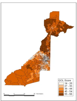
Figure 3 shows the overall quality of life score map generated by the pixel-based approach. Because the values of each factor were ranked from 1 to 10 according to the relative desirability to the quality of life, the possible overall quality of life score can range from 1 to 70.
However, the best quality of life score in this study is 59 while the worst one is 1.
The highest quality of life score was found around Buckhead, the junction of Interstates 75 and 85, some portions of Roswell and Alpharetta, and the northeastern parts of Fulton County along Georgia 400 whereas the lowest quality of life score was found around the southwestern parts and the most northern parts of Fulton County and some portions of the central city of Atlanta. The areas
with the highest quality of life score are characterized by the highest median household income, the highest median home value, the higher NDVI, the lower surface temperature, very high percentage of college graduates, lower population density, and lower percentage of urban use. In contrast, the places with the lowest quality of life score are characterized by lower median household income, lower median home value, and lower percentage of college graduates. The southern half of Fulton County showed relatively lower quality of life scores than the northern half.
FIGURE 3. Urban quality of life scores by pixel-based approach
The urban quality of life score map generated by the pixel-based approach
was compared with that by a zone-based approach. In case of the zone-based approach, three environmental variables were spatially aggregated into census block groups to integrate remotely sensed data with areal socioeconomic data. Figure 4 shows the overall quality of life score map generated by the zone-based approach. In this case, the highest quality of life score is 68 while the lowest one is 14. The spatial distribution of the highest quality of life score was similar to that of the pixel-based approach, but the pixel-based approach reveals the sub-unit or microscale variation in the quality of life scores. Although the pixel-based approach costs an intermediate step such as the disaggregation of zonal data with more processing time, it facilitates integrating remotely sensed and socioeconomic data and visualizing them in the quality of life assessment. The spatial distribution of the lowest quality of life score was somewhat different from that of the pixel-based approach. The lowest quality of life score was found around the central city of Atlanta. The places with the lowest quality of life score are characterized by lower median household income, lower median home value, lower percentage of college graduates, lower NDVI, higher population density, higher surface temperature, and higher percentage of urban use. The results from the zone-based approach confirmed that the major urbanized areas and the southern half of Fulton County had relatively lower quality of life scores than their counterparts.
FIGURE 4. Urban quality of life scores by zone-based approach
Despite its advantages, there are several issues to be taken into consideration for the pixel-based approach to urban quality of life assessment. First, the pixel-based approach to urban quality of life assessment can be regarded as a spatial decision problem under the conditions of uncertainty since there is no objectively optimal solution. The cartographic modeling analysis used in this study is a subjective approach to determine the quality of life score. To complement this approach, alternative objective approaches from multicriteria evaluation techniques and multispectral remote sensing image analysis can be used to integrate and transform the seven variables into a resultant quality of life score for each pixel.
Second, the dasymetric mapping method
used to spatially disaggregate two demographic variables, population density and percent of college graduates, into individual pixels suffers from two weaknesses. In the dasymetric mapping process, the weighting percentages are subjectively determined and the differences in area among the five land use and cover classes within a census block group are not considered. An alternative approach to dasymetric mapping is needed to address the two weaknesses and improve the accuracy of the redistribution of population.
Third, it is necessary to explore the optimal cell size for the dasymetric mapping method. Since the land use and cover data derived from the Landsat TM image were initially converted to a 30-m-resolution raster grid, this grid cell size serves as the resolution for the raster population surfaces generated by the dasymetric mapping method. However, the choice of grid cell size must be made according to the computational complexity and the resolution capacity to capture the desired spatial variation of population within the area of interest.
CONCLUSION
This research demonstrated a pixel-based approach to integrating remotely sensed data and socioeconomic data for urban quality of life assessment. Two techniques were presented that spatially disaggregate areal socioeconomic data into individual pixels for the quality of life assessment. The first technique suggests a dasymetric mapping method to disaggregate areal demographic data into individual pixels. The second
technique is the use of a spatial interpolation method to disaggregate zonal economic data into individual pixels. These spatial microsimulation techniques not only assist in calculating a microscale or sub-unit indicator in the urban quality of life assessment, but also streamline the efficient integration of remotely sensed data with socioeconomic data and visualization of the two data in the assessment at the cost of more processing time. In other words, the pixel-based approach to urban quality of life assessment allows for more microscopic evaluation than is possible with the zone-based approach.
In this manner, this research implies that the pixel-based approach provides the potential for the development of new database and increased analytical capabilities in urban analysis. This methodological challenge will help to model hypothetical urban structures and to spur more socioeconomic applications with the use of remotely sensed data. This research may address a new research agenda relating to spatial microsimulation analysis within the field of geocomputation.
ACKNOWLEDGEMENT
The author is very grateful to Dr. E.
Lynn Usery for his constructive comments and suggestions on an earlier draft of this manuscript.
REFERENCES
Anderson, J.R., E.E. Hardy, J.T. Roach and R.E. Witmer. 1976. A Land use and land cover classification system for use with remote sensor data. U.S. Geological Survey
(USGS) Professional Paper 964, Sioux Falls, SD, USA. 41pp.
Bederman, S.H. and T.A. Hartshorn. 1984.
Quality of life in Georgia: the 1980 experience. Southeastern Geographer 24(2):
78-98.
Chen, K. 2002. An approach to linking remotely sensed data and areal census data.
International Journal of Remote Sensing 23(1): 37-48.
Fisher, P.F. and M. Langford. 1996. Modeling sensitivity to accuracy in classified imagery:
a study of areal interpolation by dasymetric mapping. Professional Geographer 48(3):
299-309.
Forster, B. 1983. Some urban measurements from Landsat data. Photogrammetric Engineering and Remote Sensing 49(12):
1693-1707.
Goodchild, M.F. and N.S-N. Lam. 1980. Areal interpolation: a variant of the traditional spatial problem. Geoprocessing 1: 297-312.
Liu, B.C. 1976. Quality of life indicators in U.S. metropolitan areas, 1970. Midwest Research Institute, Kansas City, MO, USA.
58pp.
Lo, C.P. and B.J. Faber. 1997. Integration of Landsat thematic mapper and census data for quality of life assessment. Remote Sensing of Environment 62: 143-157.
Martin, D. 1996. Geographic Information Systems: Socioeconomic Applications.
Routleedge, New York, NY, USA. 210pp.
Martin, D. and I. Bracken. 1993. The integration of socioeconomic and physical resource data for applied land management
information systems. Applied Geography 13:
45-53.
Mesev, V. (ed.). 2003. Remotely Sensed Cities.
Taylor & Francis, New York, NY, USA.
368pp.
Nichol, J.E. 1994. A GIS-based approach to microclimatic monitoring in Singapore’s high-rise housing estates. Photogrammetric Engineering and Remote Sensing 60(10):
1225-1232.
Smith, D.M. 1973. The Geography of Social Well-being in the United States. McGraw Hill, New York, NY, USA. 156pp.
Slocum, T.A., R.B. McMaster, F.C. Kessler and H.H. Howard. 2005. Thematic Cartography and Geographic Visualization.
Pearson Prentice Hall, Upper Saddle River, NJ, USA. 575pp.
Spiekermann, K. and M. Wegner. 2000.
Freedom from the tyranny of zones:
towards new GIS-based spatial models. In:
Fortheringham, A.S. and M. Wegner.(eds.).
Spatial Models and GIS: New Potentials and New Models. Taylor & Francis, London, UK, pp.45-61.
Wallace, S. 1971. Quality of life. Journal of Home Economics 66: 7-8.
Weber, C. and J. Hirsh. 1992. Some urban measurements from SPOT data: urban life quality indices. International Journal of Remote Sensing 13(17): 3251-3261.
Wukelic, G.E., D.E. Gibbons, L.M. Martucci and H.P. Foote. 1989. Radiometric calibration of Landsat thematic mapper thermal band. Remote Sensing of Environment 28: 339-347.