Accuracy Assessment of Topographic Volume Estimation Using Kompsat-3 and 3-A Stereo Data

(1)

Journal of the Korean Society of Surveying, Geodesy, Photogrammetry and Cartography Vol. 35, No. 4, 261-268, 2017

https://doi.org/10.7848/ksgpc.2017.35.4.261

Accuracy Assessment of Topographic Volume Estimation Using Kompsat-3 and 3-A Stereo Data

Oh, Jae-Hong

¹⁾

·Lee, Chang-No

²⁾

Abstract

The topographic volume estimation is carried out for the earth work of a construction site and quarry excavation monitoring. The topographic surveying using instruments such as engineering levels, total stations, and GNSS (Global Navigation Satellite Systems) receivers have traditionally been used and the photogrammetric approach using drone systems has recently been introduced. However, these methods cannot be adopted for inaccessible areas where high resolution satellite images can be an alternative. We carried out experiments using Kompsat-3/3A data to estimate topographic volume for a quarry and checked the accuracy. We generated DEMs (Digital Elevation Model) using newly acquired Kompsat-3/3A data and checked the accuracy of the topographic volume estimation by comparing them to a reference DEM generated by timely operating a drone system. The experimental results showed that geometric differences between stereo images significantly lower the quality of the volume estimation.

The tested Kompsat-3 data showed one meter level of elevation accuracy with the volume estimation error less than 1% while the tested Kompsat-3A data showed lower results because of the large geometric difference.

Keywords : Volume Estimation, Kompsat-3, High Resolution Satellite Images, DEM, Stereo

ISSN 1598-4850(Print) ISSN 2288-260X(Online) Original article

1. Introduction

The earth work of a construction site and the quarry excavation require the topographic volume estimation for which terrestrial surveying instruments and high resolution drone systems are used. Topographic surfaces are often represented in DEM (Digital Elevation Model) that is generated by interpolating 3D point clouds where measurements have been carried out. DEM is the most popular topographic surface model used not only for the earth volume work estimations, but hydrology analysis and the visibility analysis.

Engineering levels, total stations, and GNSS (Global Navigation Satellite Systems) receivers have traditionally been used for the topographic surveying. Recently the photogrammetric approach using drone systems has been introduced (Lee and Choi, 2016). However the conventional

methods have limitations for inaccessible areas where high resolution satellite images can be an alternative. For example, Tsutsui et al. (2007) used DEMs extracted from high- resolution satellite images to estimate the volume change due to the landslide. Bagnardi et al. (2016) studied the use of tri- stereo Pleiades-1 images to generate an one meter resolution DEM and measure a lava ﬂow volume of Fogo Volcano.

In the study, we tested Kompsat-3 data for the topographic volume estimation. Kompsat-3’s AEISS (Advanced Electronic Image Scanning System) camera produces panchromatic with 70 cm GSD (Ground Sampling Distance) and multispectral with 2.8-meter GSD. Kompsat-3A’s AEISS-A camera is similar to Kompsat-3’s AEISS but it was designed to provide slightly better spatial resolution (panchromatic 0.55 m, multispectral 2.20 m) (Seo et al., 2016). Swath widths of Kompsat-3 and Kompsat-3A are 15km and 12km at nadir, respectively. We generated DEMs using newly acquired

This is an Open Access article distributed under the terms of the Creative Commons Attribution Non-Commercial License (http://

creativecommons.org/licenses/by-nc/3.0) which permits unrestricted non-commercial use, distribution, and reproduction in any medium, provided the original work is properly cited.

Received 2017. 07. 18, Revised 2017. 08. 04, Accepted 2017. 08. 28

1) Member, Dept. of Civil Engineering, Chonnam National University (E-email: [email protected])

2) Corresponding Author, Member, Dept. of Civil Engineering, Seoul National University of Science and Technology (E-mail: [email protected])

(2)

Journal of the Korean Society of Surveying, Geodesy, Photogrammetry and Cartography, Vol. 35, No. 4, 261-268, 2017

Kompsat-3/3A data over a quarry and check the accuracy of the topographic volume estimation by comparing them to a reference DEM generated by timely operating a drone system with GNSS control surveying.

2. Methodology

For the study, we newly acquired Kompsat-3 and 3A stereo images over the test site. Then Kompsat-3 data were processed with typical high-resolution satellite image processing methods which include the georeferencing (i.e.

sensor modelling), the epipolar image resampling, the stereo image matching, and the reconstruction for 3D point clouds.

Finally, we performed the accuracy assessment as shown in Fig. 1.

2.1 Sensor modelling

Sensor modelling is carried out using RPCs (Rational Polynomial Coefficients) which forms the nonlinear equation.

In Eqs.(1)-(4), an image coordinates (s,l) is computed using the given 80 RPCs (a,b,c,d) from a given ground

coordinates(φ,λ,h) . For a precise stereo processing without any GCP (Ground Control Point), the relative orientation can be carried out to remove the parallax between a stereo data set. Tie points extracted over the entire image are used to reconstruct the ground coordinates to model the refinement parameters (A

₀

, A

₁

,..., B

₂

).

( ) ,sl

( a b c d , , , ) ( ϕ λ , ,h )

( A A

0

, ,...,

1

B

2

)

( ) ( )

0 1 2 1 2

0 1 2 3 4

, , , ,

l A Al A s F U V W F U V W s B B l B s F U V W F U V W

+ + + =

+ + + = ⁽¹⁾

,l s

F

i

U V ,

W . A A

₀

, ,...,

₁

B

₂

, , , ,

O O O O O

S S S S S

h h l L s S

U V W Y X

h L S

ϕ ϕ λ λ

ϕ λ

− − − − −

= = = = = (2)

( )

1 2 3 4

, , , , , , , ,

T T T T

F U V W a u F U V W b u F U V W c u F U V W d u

=

(3)

[ ] [ ]

1 2 20 1 2 20

2

2 2 3 2 2 2

3 2 2 2 3

, , 1

]

T T

T

a a a a b b b b

c c c c d d d d

u V U W VU VW UW V U W UVW V VU VW V U U UW V W U W W

= =

=  

2 3

3 3

(4)

, , U V W

(1) where, l,s are line and sample coordinates and

( ) ^,sl ( a b c d ^{, , ,} ) ( ^{ϕ λ} ^{, ,h} )

( A A

0

, ,...,

1

B

2

)

( ) ( )

0 1 2 1 2

0 1 2 3 4

, , , ,

l A Al A s F U V W F U V W s B B l B s F U V W F U V W

+ + + =

+ + + = (1)

,l s

F

i

, U V

W . A A

₀

, ,...,

₁

B

₂

, , , ,

O O O O O

S S S S S

h h l L s S

U V W Y X

h L S

ϕ ϕ λ λ

ϕ λ

− − − − −

= = = = = (2)

( )

1 2 3 4

, , , , , , , ,

T T T T

F U V W a u F U V W b u F U V W c u F U V W d u

=

(3)

[ ] [ ]

1 2 20 1 2 20

2

2 2 3 2 2 2

3 2 2 2 3

, , 1

]

T T

T

a a a a b b b b

c c c c d d d d

u V U W VU VW UW V U W UVW V VU VW V U U UW V W U W W

= =

=  

2 3

3 3

(4)

, , U V W

are third- order polynomial functions of object space coordinates

( ) ,sl

( a b c d ^{, , ,} ) ( ^{ϕ λ} ^{, ,h} )

( A A

0

, ,...,

1

B

2

)

( ) ( )

0 1 2 1 2

0 1 2 3 4

, , , ,

l A Al A s F U V W F U V W s B B l B s F U V W F U V W

+ + + =

+ + + = (1)

,l s

F

i

, U V

W . A A

₀

, ,...,

₁

B

₂

, , , ,

O O O O O

S S S S S

h h l L s S

U V W Y X

h L S

ϕ ϕ λ λ

ϕ λ

− − − − −

= = = = = (2)

( )

1 2 3 4

, , , , , , , ,

T T T T

F U V W a u F U V W b u F U V W c u F U V W d u

=

(3)

[ ] [ ]

1 2 20 1 2 20

2

2 2 3 2 2 2

3 2 2 2 3

, , 1

]

T T

T

a a a a b b b b

c c c c d d d d

u V U W VU VW UW V U W UVW V VU VW V U U UW V W U W W

= =

=  

2 3

3 3

(4)

, , U V W

and

( ) ,sl

( a b c d ^{, , ,} ) ( ϕ λ , ,h )

( A A

0

, ,...,

1

B

2

)

( ) ( )

0 1 2 1 2

0 1 2 3 4

, , , ,

l A Al A s F U V W F U V W s B B l B s F U V W F U V W

+ + + =

+ + + = (1)

,l s

F

i

U V ,

W . A A

₀

, ,...,

₁

B

₂

, , , ,

O O O O O

S S S S S

h h l L s S

U V W Y X

h L S

ϕ ϕ λ λ

ϕ λ

− − − − −

= = = = = (2)

( )

1 2 3 4

, , , , , , , ,

T T T T

F U V W a u F U V W b u F U V W c u F U V W d u

=

(3)

[ ] [ ]

1 2 20 1 2 20

2

2 2 3 2 2 2

3 2 2 2 3

, , 1

]

T T

T

a a a a b b b b

c c c c d d d d

u V U W VU VW UW V U W UVW V VU VW V U U UW V W U W W

= =

=  

2 3

3 3

(4)

, , U V W

( ) ,sl

( a b c d ^{, , ,} ) ( ϕ λ , ,h )

( A A

0

, ,...,

1

B

2

)

( ) ( )

0 1 2 1 2

0 1 2 3 4

, , , ,

l A Al A s F U V W F U V W s B B l B s F U V W F U V W

+ + + =

+ + + = (1)

,l s

F

i

U V ,

W . A A

₀

, ,...,

₁

B

₂

, , , ,

O O O O O

S S S S S

h h l L s S

U V W Y X

h L S

ϕ ϕ λ λ

ϕ λ

− − − − −

= = = = = (2)

( )

1 2 3 4

, , , , , , , ,

T T T T

F U V W a u F U V W b u F U V W c u F U V W d u

=

(3)

[ ] [ ]

1 2 20 1 2 20

2

2 2 3 2 2 2

3 2 2 2 3

, , 1

]

T T

T

a a a a b b b b

c c c c d d d d

u V U W VU VW UW V U W UVW V VU VW V U U UW V W U W W

= =

=  

2 3

3 3

(4)

, , U V W

describe an refinement parameters.

( a b c d , , , ) ( ϕ λ , ,h )

( A A

0

, ,...,

1

B

2

)

( ) ( )

0 1 2 1 2

0 1 2 3 4

, , , ,

l A Al A s F U V W F U V W s B B l B s F U V W F U V W

+ + + =

+ + + = (1)

,ls

F

i

, U V

W . A A

₀

, ,...,

₁

B

₂

, , , ,

O O O O O

S S S S S

h h l L s S

U V W Y X

h L S

ϕ ϕ λ λ

ϕ λ

− − − − −

= = = = = (2)

( )

1 2 3 4

, , , , , , , ,

T T T T

F U V W a u F U V W b u F U V W c u F U V W d u

=

(3)

[ ] [ ]

1 2 20 1 2 20

2

2 2 3 2 2 2

3 2 2 2 3

, , 1

]

T T

T

a a a a b b b b c c c c d d d d u V U W VU VW UW V

U W UVW V VU VW V U U UW V W U W W

= =

=  

2 3

3 3

(4)

, , U V W

(2)

( a b c d ^{, , ,} ) ( ^{ϕ λ} ^{, ,h} )

( A A

0

, ,...,

1

B

2

)

( ) ( )

0 1 2 1 2

0 1 2 3 4

, , , ,

l A Al A s F U V W F U V W s B B l B s F U V W F U V W

+ + + =

+ + + = (1)

,l s

F

i

, U V

W . A A

₀

, ,...,

₁

B

₂

, , , ,

O O O O O

S S S S S

h h l L s S

U V W Y X

h L S

ϕ ϕ λ λ

ϕ λ

− − − − −

= = = = = (2)

( )

1 2 3 4

, , , , , , , ,

T T T T

F U V W a u F U V W b u F U V W c u F U V W d u

=

(3)

[ ] [ ]

1 2 20 1 2 20

2

2 2 3 2 2 2

3 2 2 2 3

, , 1

]

T T

T

a a a a b b b b

c c c c d d d d

u V U W VU VW UW V U W UVW V VU VW V U U UW V W U W W

= =

=  

2 3

3 3

(4)

, , U V W

(3)

( a b c d , , , ) ( ϕ λ , ,h )

( A A

0

, ,...,

1

B

2

)

( ) ( )

0 1 2 1 2

0 1 2 3 4

, , , ,

l A Al A s F U V W F U V W s B B l B s F U V W F U V W

+ + + =

+ + + = (1)

,l s

F

i

, U V

W . A A

₀

, ,...,

₁

B

₂

, , , ,

O O O O O

S S S S S

h h l L s S

U V W Y X

h L S

ϕ ϕ λ λ

ϕ λ

− − − − −

= = = = = (2)

( )

1 2 3 4

, , , , , , , ,

T T T T

F U V W a u F U V W b u F U V W c u F U V W d u

=

(3)

[ ] [ ]

1 2 20 1 2 20

2

2 2 3 2 2 2

3 2 2 2 3

, , 1

]

T T

T

a a a a b b b b

c c c c d d d d

u V U W VU VW UW V U W UVW V VU VW V U U UW V W U W W

= =

=  

2 3

3 3

(4)

U V W, ,

(4)

where,

( a b c d ^{, , ,} ) ( ϕ λ , ,h )

( A A

0

, ,...,

1

B

2

)

( ) ( )

0 1 2 1 2

0 1 2 3 4

, , , ,

l A Al A s F U V W F U V W s B B l B s F U V W F U V W

+ + + =

+ + + = (1)

,l s

F

i

U V ,

W . A A

₀

, ,...,

₁

B

₂

, , , ,

O O O O O

S S S S S

h h l L s S

U V W Y X

h L S

ϕ ϕ λ λ

ϕ λ

− − − − −

= = = = = (2)

( )

1 2 3 4

, , , , , , , ,

T T T T

F U V W a u F U V W b u F U V W c u F U V W d u

=

(3)

[ ] [ ]

1 2 20 1 2 20

2

2 2 3 2 2 2

3 2 2 2 3

, , 1

]

T T

T

a a a a b b b b

c c c c d d d d

u V U W VU VW UW V U W UVW V VU VW V U U UW V W U W W

= =

=  

2 3

3 3

(4)

, , U V W

the normalized object space coordinates of ground target; ^{φ λ} ^{, ,h}

,l s

0, , , ,0h S L0 0 0

φ λ

, , , ,

S S

h S L

S S S

φ λ

( )( ) ( )

²

( )

²

1 1 1 1 1 1

w w w w w w

ij ij ij ij

i j i j i j

ncc L L R R L L R R

= = = = = =

   

 

= ∑∑  − −    ∑∑ −     ∑∑ −   ⁽⁵⁾

w w × ;

L R,

the geodetic latitude, longitude and ellipsoidal height of ground target;

φ λ , ,h ,l s

0, , , ,0h S L0 0 0

φ λ

, , , ,

S S

h S L

S S S

φ λ

( )( ) ( )

²

( )

²

1 1 1 1 1 1

w w w w w w

ij ij ij ij

i j i j i j

ncc L L R R L L R R

= = = = = =

   

 

= ∑∑  − −    ∑∑ −     ∑∑ −   ⁽⁵⁾

w w × ;

, L R

the image line (row) and sample (column) coordinates;

φ λ , ,h ,l s

0, , , ,0h S L0 0 0

φ λ

, , , ,

S S

h S L

S S S

φ λ

( )( ) ( )

²

( )

²

1 1 1 1 1 1

w w w w w w

ij ij ij ij

i j i j i j

ncc L L R R L L R R

= = = = = =

   

 

= ∑∑  − −    ∑∑ −     ∑∑ −   ⁽⁵⁾

w w × ;

, L R

∑ ⁻ ⁺

i i i

T

R_, ₎

M RD T

²

(

( )

min

the offset factors for the latitude, longitude, height, sample and line;

, ,h φ λ

,l s

0, , , ,0h S L0 0 0

φ λ

, , , ,

S S

h S L

S S S

φ λ

( )( ) ( )

²

( )

²

1 1 1 1 1 1

w w w w w w

ij ij ij ij

i j i j i j

ncc L L R R L L R R

= = = = = =

   

 

= ∑∑  − −    ∑∑ −     ∑∑ −   ⁽⁵⁾

w w × ;

, L R

∑ ⁻ ⁺

i i i

T

R_, ₎

M RD T

²

(

( )

min

the scale factors for the latitude, longitude, height, sample and line.

2.2 Epipolar image generation

For the epipolar image generation, the epipolar curve

points are piecewisely generated as depicted in Fig. 2. The

projection through the left image, the ground, and the right

image is carried out iteratively to obtain the curve point set

constituting an epipolar curve. In the projection, the elevation

range can be obtained from RPCs. The interval between the

Fig. 1. Flowchart of the study

(3)

Accuracy Assessment of Topographic Volume Estimation Using Kompsat-3 and 3-A Stereo Data

curves can be established manually such as 1/10 or 1/20 of the image size. Next the epipolar curve points are rearranged to satisfy the epipolar resampled image conditions that include zero y-parallax and the linear relationship between the x-parallax and the ground height (Oh et al., 2010).

2.3 Stereo matching

The stereo matching is carried out with the image pyramids generated from stereo images for efficiency. The stereo matching begins at the lowest level of the image pyramid and proceeds to upper levels reducing the search range along x-direction. In addition, the matching is performed along the epipolar line to limit the search range along y-direction. The similarity measure can be simply carried out to find the best location in the right image using NCC (Normalized Cross Correlation) in Eq.(5).

, ,h φ λ

,ls

0 0 0 0 0, , , ,h S L φ λ

, , , ,

S S S

h S L

S S

φ λ

( )( ) ( )

²

( )

²

1 1 1 1 1 1

w w w w w w

ij ij ij ij

i j i j i j

ncc L L R R L L R R

= = = = = =

   

 

= ∑∑  − −    ∑∑ −     ∑∑ −   ⁽⁵⁾ w w × ;

,LR

∑ ⁻ ⁺

i i i

T

R_,₎

M RD T

²

(

( )

min

(5)

where, L is an image patch from the left epipolar image, and R is a right image patch within the search region, both are in the size of

, ,h φ λ

,l s

0, , , ,0 h S L0 0 0

φ λ

, , , ,

S S

h S L

S S S

φ λ

( )( ) ( )

²

( )

²

1 1 1 1 1 1

w w w w w w

ij ij ij ij

i j i j i j

ncc L L R R L L R R

= = = = = =

   

 

= ∑∑  − −    ∑∑ −     ∑∑ −   ⁽⁵⁾

w w × ;

L R,

∑ ⁻ ⁺

i i i

T

R_, ₎

M RD T

²

(

( )

min

; φ λ , ,h

,l s

0, , , ,0h S L0 0 0

φ λ

, , , ,

S S

h S L

S S S

φ λ

( )( ) ( )

²

( )

²

1 1 1 1 1 1

w w w w w w

ij ij ij ij

i j i j i j

ncc L L R R L L R R

= = = = = =

   

 

= ∑∑  − −    ∑∑ −     ∑∑ −   ⁽⁵⁾

w w × ;

, L R

∑ ⁻ ⁺

i i i

T

R_, ₎

M RD T

²

(

( )

min

average of all intensity value within the image patches.

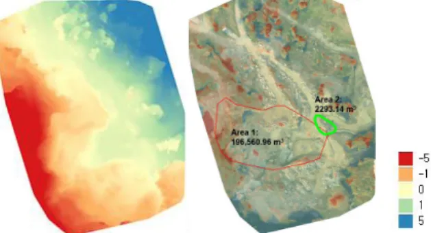
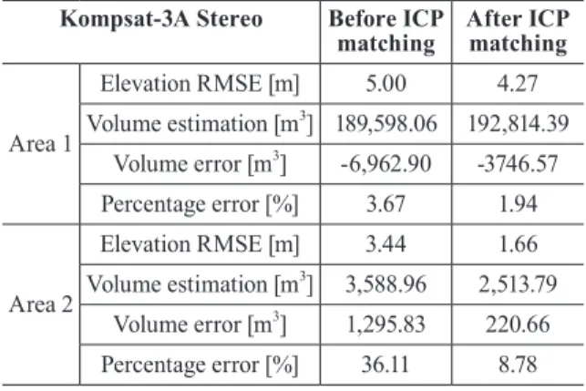
2.4 Bias removal for accuracy assessment The georeferencing without GCP produces positional biases in the resulted DEM. Therefore the volume estimation accuracy should be checked after the bias removal process. To this end the ICP (Iterative Closest Point) matching algorithm (Zhang, 1994) can be used. This is a registration method for

2D or 3D point cloud data sets by finds the closest points between two point sets. The reference is fixed while the input data is transformed to best match the reference. A 3D rigid body transformation estimation is typically applied between the corresponding point sets to determine translations and rotations iteratively. The ICP matching can be expressed in the following:

, ,h φ λ

,l s

0, , , ,0h S L0 0 0

φ λ

, , , ,

S S

h S L

S S S

φ λ

( )( ) ( )

²

( )

²

1 1 1 1 1 1

w w w w w w

ij ij ij ij

i j i j i j

ncc L L R R L L R R

= = = = = =

   

 

= ∑∑  − −    ∑∑ −     ∑∑ −   ⁽⁵⁾

w w × ;

, L R

∑ ⁻ ⁺

i i i

T

R_, ₎

M RD T

²

(

( )

min (6)

Where R = 3x3 rotation matrix, T = 3x1 translation vector, M = model (target), D = point data, and i = point index

3. Experiment

3.1 Test data

Kompsat-3 and 3A stereo data were newly acquired in 13~14 PM (local) Nov 2, 2016 and Nov 15, 2016 respectively over the test site as shown in Table 1. The data were acquired with the along-track stereo in the strip imaging mode. The product level is Level 1R which is radiometrically corrected, but not geometrically corrected.

First we computed the convergence angle, assymmetry

and BIE(bisector) angles to estimate the quality of the stereo

data (Jeong and Kim, 2016). Convergence angles mainly

affect the elevation quality and angles with less than 15

degrees considerably lower the elevation precision of the

target. Therefore, higher angles than 30 degrees are favoured

but too large angle may lower the match rate due to the large

geometric difference between stereo data. Assymmetry

and BIE angles usually affect horizontal coordinate quality

such that asymmetry angle of less than 10 degrees and BIE

Fig. 2. The epipolar curve generation (Oh et al., 2010)

(4)

angle of larger than 70 degrees are preferred (zero degrees of asymmetry and 90 degrees of BIE are ideal). Kompsat-3 satisfies the aforementioned conditions but Kompsat-3A data show too large convergence angle and low BIE angle indicating that there can be large geometric difference between the images.

We subset the area of interest from the entire scene and the images are shown in

Fig. 3. For spatial resolution reference a rock is about 2m in diameter in the aerial image. The data acquisition was made around 13~14 PM in the sunny day that quite strong shadow can be observed along the steep slopes. Note that Kompsat- 3A data have large incidence angles resulting in a poor image quality compared to Kompsat-3 data.

3.2 Stereo processing for DEM

Kompsat-3 and 3A data were resampled for epipolar images where conjugate point pairs align in the same image line not only to minimize the negative effects of matching outliers but also to increase the matching speed by significantly reducing the search area. Fig. 4 show the results of the epipolar image resampling for each data. In the overlapped epipolar image, we can observe large geometric difference between the Kompsat-3A stereo set.

The stereo matching was carried out with four levels of the image pyramid generated with the Gaussian filtering considering the image size. We used typical correlation thresholds such as 0.7 for the similarity measure and 7×7 pixels for the matching window size. The height range of the test site is set to 50m to 250m. Table 2 shows total 610,824 points were matched for Kompsat-3 stereo data showing 71.2% match rate while Kompsat-3A showed only 27.9% of match rate. The significant geometric discrepancy between Kompsat-3A undermined the matching performance. In Fig.

5, the sparse matching point distribution in Kompsat-3A can be seen compared to the case of Kompsat-3.

Table 1. Speciﬁcation of Kompsat-3 test data

Kompsat-3 Kompsat-3A

Processing level Level 1R Level 1R Acquisition date

and time

Nov 2, 2016 13:30:45 (Local) 13:31:59 (Local)

Nov 15, 2016 13:50:26 (Local) 13:51:57 (Local) Incidence/

Azimuth 22.287 /168.992 deg

22.395 /345.003 deg 35.744 /193.627 deg 37.302 /325.171 deg Convergence

Asymmetry BIE angles

44.6 deg 0.005 deg

89.2 deg

65.7 deg 0.89 deg 73.1 deg GSD (line/

sample) 0.81m/0.76m

0.81m/0.76m 0.75m/0.65m 0.79m/0.71m

Fig. 3. Left (drone images: Nov 3

^rd

), middle(Kompsat-3:

Nov 2

^nd

), right(Kompsat-3A: Nov 15

^th

)

Fig. 4. Epipolar image generation for Kompsat-3(up) and

Kompsat-3A(bottom) stereo data

(5)

Accuracy Assessment of Topographic Volume Estimation Using Kompsat-3 and 3-A Stereo Data

The match points were used to reconstruct the ground point clouds through the space intersection of stereo RPCs.

The point clouds were interpolated for 1m spatial resolution DEMs as shown in Fig. 6. Though Kompsat-3A showed the low match rate, DEM was interpolated in one meter for the comparison.

3.3 Accuracy analysis

We carried out a photogrammetric surveying using a drone over the test site on Nov 3, 2016 which is one day after Kompsat-3 stereo data acquired. This is to generate a timely reference DEM for the accuracy analysis. DJI Phantom 4 was used for 47 aerial images acquisition. The drone was operated with approximate altitude 100m above the ground and produced 3.67cm GSD images. To photogrammetrically

process the acquired images, 8 GCPs were surveyed using GNSS in the network RTK(Real Time Kinematic) mode.

The bundle adjustment was carried out with automatically generated tie points (mean 19,835 points per image) and manually measured GCPs. The interior orientation parameters were estimated on the ﬂy. The residuals in RMSE (Root Mean Square Error) of the bundle adjustment at GCP are shown in Table 3.

Fig. 7 shows the generated DEM that total 3,338,789 points were used for the DEM resulting in average point density of 55 points per m

³

. We carried out a simple difference between Kompsat-3 DEM and the reference DEM for the coloured difference image in the right. The positive value indicates that Kompsat-3 DEM is estimated higher than the reference.

Note that along the steep slope locate the large errors. This is because lower scale DEMs tend to smooth out the steep slope.

We computed the volume estimation for area 1 and area 2 shown in Fig. 7 by setting the horizontal plane of the minimum elevation of each reference data. Horizontal area of area 1 and area 2 are 10,509m

²

, 417m

²

, respectively and this means that one-meter elevation bias in a DEM can be resulted in the volume error of 10,509m

³

, 417m

³

, for each area.

Fig. 5. Stereo image matching point distribution Table 2. Stereo match rate

Number of match points Kompsat-3 Kompsat-3A

Matched points 610,824 183,573

Match rate 71.2% 27.9%

Fig. 6. Generated DEMs

Table 3. The residual of the aerial image bundle adjustment

RMSE at GCPs

East / North 4.3cm / 4.7cm

Elevation 7.5cm

Fig. 7. Reference DEM and the differenced DEM with

Kompsat-3 DEM

(6)

In the study, the satellite images were not accurately georeferenced and this produces systematic bias in the resulted topographic data. The bias prevents from the reliable volume accuracy assessment so that we applied ICP matching to fit the resulted DEMs to the reference for the bias correction. This enables the better identification of local geometric discrepancy of the resulted DEMs. Fig. 8 shows the ICP matching between the Kompsat-3 DEM (red dots) and the reference DEM (blue dots) for area 2. After 11 iterations, the Kompsat-3 DEM was transformed to the green triangles which fit the reference.

Table 4 shows the estimated volumes and their errors of Kompsat-3 DEM. The elevation errors of the DEM are 2.09m, 1.48m in RMSE before and after the ICP matching, respectively. The volume of area 1 was estimated 205,058.30m

³

, 195,411.56m

³

respectively. The volume estimation error decreased from 8,497.34 to -1,149.40 m

³

after

the ICP matching. Kompsat-3 estimated the volume of area 2 as 3,017.44m

³

with error of 724.30m

³

, but the estimation was 2,309.08m

³

with error of 15.94m

³

after the ICP matching.

Table 5 shows the analysed statistics for Kompsat-3A DEM. The elevation errors of the DEM are 5.00m, 4.27m in RMSE before and after the ICP matching, respectively.

Note that the data showed much larger geometric difference between the stereo resulting the less accurate matching results. The estimated volume of area 1 was 189,598m

³

and 192,814.39m

³

respectively and the estimation error decreased from -6,962.90 to -3,746.57 m

³

after the ICP matching. For area 2, Kompsat-3 estimated the volume as 3,588.96m

³

with error of 1,295.83m

³

and the estimation was 2,513.79 m

³

with error of 220.66m

³

after the ICP matching.

4. Conclusion

We tested Kompsat-3 and Kompsat-3A for the topographic volume estimation and carried out the accuracy assessment.

Kompsat-3/3A stereo data were processed with the relative orientation, the epipolar image resampling, and the stereo matching for DEMs. We compared the result to a reference DEM generated by timely operating a drone system. We checked the accuracy for two cases of before and after the bias removal process because the orientation without GCP produces positional biases in the resulted DEMs. The experimental results showed that geometric differences between stereo images significantly lower the quality of the volume estimation. The tested Kompsat-3 data showed one meter level of elevation accuracy with the volume estimation Fig. 8. Before and after the ICP matching (Kompsat-3)

Table 4. Volume estimation accuracy (Kompsat-3 stereo) Kompsat-3 Stereo Before ICP

matching After ICP matching Area 1

Elevation RMSE [m] 2.09 1.48 Volume estimation [m

³

] 205,058.30 195,411.56

Volume error [m

³

] 8,497.34 -1,149.40 Percentage error [%] 4.14 0.59 Area 2

Elevation RMSE [m] 2.12 1.05 Volume estimation [m

³

] 3,017.44 2,309.08

Volume error [m

³

] 724.30 15.94 Percentage error [%] 24.00 0.69

Table 5. Volume estimation accuracy (Kompsat-3A stereo) Kompsat-3A Stereo Before ICP

matching After ICP matching Area 1

Elevation RMSE [m] 5.00 4.27 Volume estimation [m

³

] 189,598.06 192,814.39

Volume error [m

³

] -6,962.90 -3746.57 Percentage error [%] 3.67 1.94 Area 2

Elevation RMSE [m] 3.44 1.66 Volume estimation [m

³

] 3,588.96 2,513.79

Volume error [m

³

] 1,295.83 220.66

Percentage error [%] 36.11 8.78

(7)

Accuracy Assessment of Topographic Volume Estimation Using Kompsat-3 and 3-A Stereo Data

error less than 1% while the tested Kompsat-3A data showed lower results because of the large geometric difference. The experimental results showed that Kompsat-3/3A stereo data have potentials for the topographic surveying for inaccessible areas. Future studies include accurate topographic volume change estimations using two stereo Kompsat-3 data acquired over different times.

Acknowledgment

This study was supported by Korea Aerospace Research Institute grant (FR17720W02) and National Research Foundation of Korea grant (NRF-2016R1D1A3B03930660).

References

Bagnardi, M., Gonzalez, P., and Hooper, A. (2016), High- resolution digital elevation model from tri-stereo Pleiades-1 satellite imagery for lava ﬂow volume estimates at Fogo Volcano, Geophysical Research Letters, Vol. 43, No. 12, pp. 6267-6275.

Jeong, J.H. and Kim, T.J. (2016), Quantitative estimation and validation of the effects of the convergence, bisector elevation, and asymmetry angles on the positioning accuracies of satellite stereo pair, Photogrammetric Engineering & Remote Sensing, Vol. 82, No. 8, pp. 625- 633.

Lee, S. and Choi, Y. (2016), Comparison of topographic surveying results using a fixed-wing and a popular rotary-wing unmanned aerial vehicle (drone), Tunnel &

Underground Space, Vol. 26, No. 1, pp. 24-31. (in Korean with English abstract)

Oh, J.H., Lee, W.H., Toth, C.K., Grejner-Brzezinska, D.A., and Lee, C.H. (2010), A piecewise approach to epipolar resampling of pushbroom satellite images based on RPC, Photogrammetric Engineering & Remote Sensing, Vol. 76, No. 12, pp. 1353-1363.

Seo, D., Oh, J., Lee, C., Lee, D., and Choi, H. (2016), Geometric calibration and validation of Kompsat-3A AEISS-A camera, Sensors, Vol. 16, No. 10, p. 1776.

Tsutsui, K., Rokugawa, S., Nakagawa, H., Miyazaki, S., Cheng, C., Shiraishi, T., and Yang, S. (2007), Detection and volume estimation of large landslides based on elevation- change analysis using DEMs extracted from high- resolution satellite stereo imagery, IEEE Transactions on Geoscience and Remote Sensing, Vol. 45, NO. 6, pp. 1681- 1696.

Zhang, Z. (1994), Iterative point matching for registration of

free-form curves and surfaces, International Journal of

Computer Vision, Vol. 13, No. 2, pp. 119-152.

(8)