Voltage Sag and Swell Estimation Using ANFIS for Power System Applications
N. Malmurugan·Devarajan Gopal*·Young Hwan Lho
1. Introduction
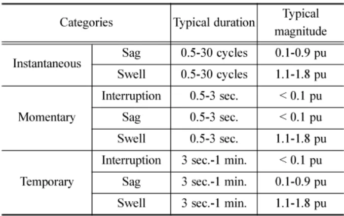
Power quality has become a main area of interest in the power engineering research community. Voltage sags and swells cause severe damage to the subsystems of power sys- tems and can subsequently bring the entire power system to halt mode. Voltage sag is a decrease to between 0.1 and 0.9 pu in RMS (Root Mean Square) voltage or current at the power frequency for a duration of 0.5 cycles to 1 minute and voltage swell is an increase to between 1.1 pu and 1.8 pu in RMS volt- age or current at a power frequency duration from 0.5 to 1 minute [1]. Table 1 shows the categories and characteristics of power system electromagnetic phenomena [2]. These sags and swells are mainly due turn on/turn off operations of supply lines and flow of inrush current during starting of different loads, etc. [2]. Turn on/turn off can happen either from the sup- ply or load side. In addition, lightning strikes and EMI (elec- tromagnetic interference) can cause momentary acceleration of sags/swells. Numerous solutions have been proposed to mit- igate sags and swells, including use of a dynamic voltage restorer that injects voltage in series with supply lines when any sags or swells are detected. Experimental investigation of voltage sag mitigation by an advanced static Var compensator has been extensively
discussed in [3]. The RMS voltage mea-surement method is generally used to detect sag and swell before any mitigation technique is employed. The main draw- back of the RMS voltage measurement is that the RMS voltage
is measured through voltage sensors and fed to the ADC of the microcontroller or DSP to be converted into a digital signal, and the data that are used are therefore based on old data that are system dependent.
The disadvantages associated with the RMS method are dis- cussed in [4-5]. Also, power quality surveys show that voltage sags are considered the dominant factor affecting power quality [6]. Rapid sag detection [7] has been achieved through the use of a nonlinear adaptive filter. The authors reported that the fil- ter can track the amplitude of the sag in real time, which would be highly useful for sag and swell mitigation. Comparisons of statistical methods and wavelet energy coefficients for deter- mining two common PQ disturbances of sag and swell are pre- sented in [8]. A novel sag detection method [9] for a line- interactive dynamic voltage restorer (DVR) has also been pre- sented. However, none of the authors used ANFIS (Adaptive Network based Fuzzy Inference System) with different mem- bership function types that can detect the RMS voltage in real Abstract
Power quality is a term that is now extensively used in power systems applications, and in this context the volt- age, current, and phase angle are discussed widely. In particular, different algorithms that are capable of detecting the volt- age sag and swell information in a real time environment have been proposed and developed. Voltage sag and swell play an important role in determining the stability, quality, and operation of a power system. This paper presents ANFIS (Adaptive Network based Fuzzy Inference System) models with different membership functions to build the voltage shape with the knowledge of known system parameters, and detect voltage sag and swell accurately. The performance of each method has been compared with each other/other methods to determine the effectiveness of the different models, and the results are pre- sented.Keywords
: Voltage sag and swell, ANFIS, Power quality, Power system applications*Corresponding author.
Tel.: +91-94437-78825, E-mail: [email protected]
©
The Korean Society for Railway 2013 http://dx.doi.org/10.7782/JKSR.2013.16.4.272
Table 1 Characteristics of electromagnetic phenomena of power systems
Categories Typical duration Typical magnitude
Instantaneous Sag 0.5-30 cycles 0.1-0.9 pu Swell 0.5-30 cycles 1.1-1.8 pu
Momentary
Interruption 0.5-3 sec. < 0.1 pu Sag 0.5-3 sec. < 0.1 pu Swell 0.5-3 sec. 1.1-1.8 pu
Temporary
Interruption 3 sec.-1 min. < 0.1 pu
Sag 3 sec.-1 min. 0.1-0.9 pu
Swell 3 sec.-1 min. 1.1-1.8 pu
time if the voltage system amplitude and frequency are known.
The present paper discusses different methods to alter the volt- age shape and then to detect voltage sags and swells at dif- ferent operating conditions. In addition, a description of ANFIS and voltage sag and swell detection algorithms are pre- sented, and the results of performance evaluations of different methods are compared.
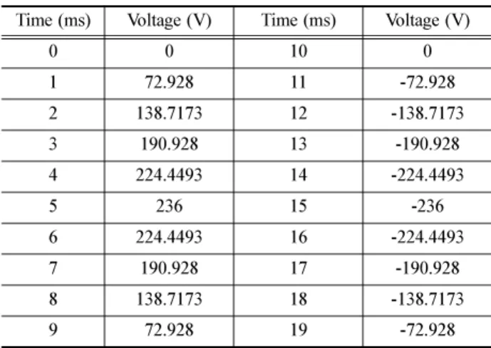
2. Necessity of Initial Voltage Measurement Voltage measurement is an essential step to develop a math- ematical model for the voltage profile. A 3 phase power quality analyzer was used to measure the voltage over one electrical cycle, which can then be employed to model different math- ematical equations. The measured voltage for two electrical cycles is shown in Fig. 1 and the corresponding data are shown in Table 2. Voltage was recorded for a 5 minute duration and the results are shown in Fig. 2.
Fig. 1 Voltage for two electrical cycles
Fig. 2 Voltage RMS for 5 min.
3. Adaptive Network Based Fuzzy Inference System
ANFIS refers to the Sugeno Adaptive Network Based Fuzzy Inference System (ANFIS) [10]. Here, the fuzzy inference sys-
tem under consideration has two inputs, time (t) and voltage ( V), and one-output predicted voltage (V
P). Each input has nine membership functions. The rule base contains eighty fuzzy Takagi and Sugeno type if-then rules. The corresponding ANFIS architecture is shown in Fig. 3.
Fig. 3 Structure of ANFIS
The ANFIS network is formed with five layers. Explanations of the layers are respectively given below.
Layer 1: In this layer, each input has 9 membership func- tions. The output of input membership function 1 is O
k1= µA
k(t) and the output of input membership function 2 is O
k2= µB
k( t), where time and voltage are the inputs. A
kand B
kare the linguistic labels (mf
1, mf
2,…, mf
9) associated with the node functions.
The output of the input membership functions specifies the variables of the t and V, and satisfies the quantifier A
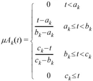
k. In this work the triangular shaped membership function µA
k(t) is used with a maximum equal to 1 and a minimum equal to 0. The generalized triangular membership function of the flux linkage is given by
Table 2 Voltage from real time measurement
Time (ms) Voltage (V) Time (ms) Voltage (V)
0 0 10 0
1 72.928 11 -72.928
2 138.7173 12 -138.7173
3 190.928 13 -190.928
4 224.4493 14 -224.4493
5 236 15 -236
6 224.4493 16 -224.4493
7 190.928 17 -190.928
8 138.7173 18 -138.7173
9 72.928 19 -72.928
(1)
Similarly, the generalized triangular shaped membership function of the current is given by
(2)
where a
k, b
k, and c
kare adaptable variables known as param- eters. As the values of these parameters change, the triangular shaped functions vary accordingly, thus exhibiting various forms of membership functions.
Layer 2: It implements the fuzzy AND operator, as in Eq.
(3).
(3)
where k = 1, 2,…, 9
Layer 3: It acts to scale or normalize the firing strengths, as shown in Eq. (4).
(4)
Layer 4: The output of the fourth layer comprises a linear combination of the inputs multiplied by the normalized firing strength. The output of this layer is given by Eq. (5).
(5)
where is the output of layer 3 and the modifiable variables m
k, n
kand r
kare known as consequent parameters.
Layer 5: Layer 5 is a simple summation of the outputs of layer 4. The overall output gives the rotor position ( θ).
(6)
4. Sag/Swell Detection Algorithm
Each algorithm has respective capabilities to predict the volt- age and is used to detect voltage sags and swells very quickly.
The step by step procedure for detecting the sag and swell is presented below and a corresponding flow chart is given in Fig. 4.
1) Start the algorithm for sag and swell
2) Identify the zero crossing point of the voltage 3) If the voltage magnitude is positive, then move to step 4, else go to step 1
4) Start the counter count = count + 1
5) If the counter reaches the max value, reset the counter and move to step 4, else go to step 6
6) Implement any one of the following functions 7) Calculate the sag/swell as per Table 1 and display the results
Fig. 4 Sag/swell detection algorithm
5. Results and Discussion
The ANFIS models have been developed by MATLAB/
Simulink, wherein input and output data are fed to the ANFIS model. Initially we considered a 9×9 triangular membership
µAkt()0 t a< k t a– k bk–ak
--- ak≤t b< k ck–t
ck–bk
--- bk≤t c< k 0 ck≤t
⎩⎪
⎪⎪
⎪⎨
⎪⎪
⎪⎪
⎧
=
µBkt()
0 V a< k V a– k bk–ak
--- ak≤V b< k ck–V
ck–bk
--- bk≤V c< k 0 ck≤V
⎩⎪
⎪⎪
⎪⎨
⎪⎪
⎪⎪
⎧
=
Wk=µAkt() µB× k( )v
Wk Wk Wk
k 1=
∑
9---
=
Ok4=Wkfk=Wk(mkt n+ kV r+ k) Wk
Ok5
∑
Wkfk Wkfk∑
kWk
∑
k---
= =
function and obtained the results. The rule viewer and surface viewer for the 9×9 membership function are presented in Fig.
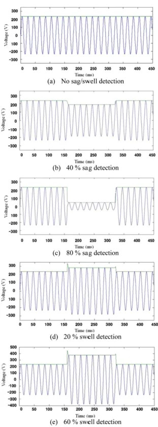
5 (a) and (b), respectively. Voltage RMS of 236V for different degrees of voltage sags/swells are shown in Fig. 6 (a)-(e).
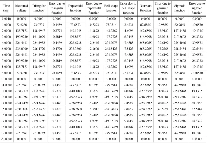
Similarly, 9×9 membership functions of trapezoidal, bell, gaussian, and sigmoid functions have been implemented and the results were obtained. From the results, the 9×9 triangular membership function outperforms all other membership func- tions, and the results are presented in Table 3. For example, when the time is 8 msecs and the input voltage is 138.71 volts, the absolute error computed by ANFIS using the triangular membership function is -0.2774. Similarly, for ANFIS using 9×9 membership functions using trapezoidal, bell, gaussian, and sigmoid functions, absolute error of -1.3872, -4.6096, -18.9423, and -19.1315, respectively, is produced. The results of all other inputs are shown in Table 1, and the absolute volt-
age error due to triangular, trapezoidal, bell shape, gaussian, and sigmoid functions vs. time for one electrical cycle is pre- sented in Fig. 7. It is evident that ANFIS with a 9×9 triangular membership function outperformed all other functions, as shown in Table 3 and Fig. 7.
Fig. 5 9×9 membership function
Fig. 6 Voltage RMS of 236 V vs. time (ms)
6. Conclusion
Five membership functions with ANFIS models have been developed and presented in this paper for a single phase power system for detecting voltage sag and swells. The developed methods have been compared with each other/other methods to determine their respective effectiveness. This paper demon- strates the ability of predicting the voltage from the knowledge of input supply parameters.
It has been observed that triangular and trapezoidal functions perform better than the other methods, because these are sim- ple ANFIS models, thereby reducing time consumption in their implementation. Furthermore, these models can be extended to any supply system to achieve higher reliability and repeat- ability in sag and swell detection. It is also noteworthy that these models require only a few input parameters such as time, voltage, and frequency magnitude with zero crossing infor- mation. It was found that the developed algorithm detects sags and swells accurately and quickly, within 2.2 msecs.
References
[1] M.H. J. Bollen (1999) Understanding Power Quality Prob- lems: Voltage Sags and Interruptions, IEEE Press, Vol. I, NY.
[2] Roger Dugan, Surya Santoso, Mark McGranaghan, H. Beaty (2004) Electric Power Systems Quality, McGraw-Hill, NY.
[3] P. Wang, N. Jenkins, M. H. J. Bollen (1998) Experimental investigation of voltage sag mitigation by an advanced static VAr compensator IEEE Trans. Power Del., 13(4), pp. 1461- 1467.
[4] X. Xiangning, X. Yonghai, L. Lianguang (2000) Simulation and analysis of voltage sag mitigation using active series volt-
Table 3 Voltage error due to triangular, trapezoidal, bell shape, gaussian, and sigmoid functions vs. time for one electrical cycle Time(ms)
Measuted voltage
Triangular function
Error due to triangular
function
Trapezoidal function
Error due to trapezoidal
function
Bell shape function
Error due to bell shape
function
Gaussian function
Error due to gaussian function
Sigmoid function
Error due to sigmoid function 0.0010 0.0000 0.0000 0.0000 0.0000 0.0000 0.0000 0.0000 0.0000 0.0000 0.0000 0.0000 1.0000 72.9280 73.0739 -0.1459 73.6573 -0.7293 75.3514 -2.4234 82.8865 -9.9585 82.9860 -10.0580 2.0000 138.7173 138.9947 -0.2774 140.1045 -1.3872 143.3269 -4.6096 157.6596 -18.9423 157.8488 -19.1315 3.0000 190.9280 191.3099 -0.3819 192.8373 -1.9093 197.2725 -6.3445 216.9998 -26.0718 217.2602 -26.3322 4.0000 224.4493 224.8982 -0.4489 226.6938 -2.2445 231.9078 -7.4585 255.0985 -30.6492 255.4046 -30.9553 5.0000 236.0000 236.4720 -0.4720 238.3600 -2.3600 243.8423 -7.8423 268.2265 -32.2265 268.5484 -32.5484 6.0000 224.4493 224.8982 -0.4489 226.6938 -2.2445 231.9078 -7.4585 255.0985 -30.6492 255.4046 -30.9553 7.0000 190.9280 191.3099 -0.3819 192.8373 -1.9093 197.2725 -6.3445 216.9998 -26.0718 217.2602 -26.3322 8.0000 138.7173 138.9947 -0.2774 140.1045 -1.3872 143.3269 -4.6096 157.6596 -18.9423 157.8488 -19.1315 9.0000 72.9280 73.0739 -0.1459 73.6573 -0.7293 75.3514 -2.4234 82.8865 -9.9585 82.9860 -10.0580 10.0000 0.0000 0.0000 0.0000 0.0000 0.0000 0.0000 0.0000 0.0000 0.0000 0.0000 0.0000 11.0000 -72.9280 -73.0739 0.1459 -73.6573 0.7293 -75.3514 2.4234 -82.8865 9.9585 -82.9860 10.0580 12.0000 -138.7173 -138.9947 0.2774 -140.1045 1.3872 -143.3269 4.6096 -157.6596 18.9423 -157.8488 19.1315 13.0000 -190.9280 -191.3099 0.3819 -192.8373 1.9093 -197.2725 6.3445 -216.9998 26.0718 -217.2602 26.3322 14.0000 -224.4493 -224.8982 0.4489 -226.6938 2.2445 -231.9078 7.4585 -255.0985 30.6492 -255.4046 30.9553 15.0000 -236.0000 -236.4720 0.4720 -238.3600 2.3600 -243.8423 7.8423 -268.2265 32.2265 -268.5484 32.5484 16.0000 -224.4493 -224.8982 0.4489 -226.6938 2.2445 -231.9078 7.4585 -255.0985 30.6492 -255.4046 30.9553 17.0000 -190.9280 -191.3099 0.3819 -192.8373 1.9093 -197.2725 6.3445 -216.9998 26.0718 -217.2602 26.3322 18.0000 -138.7173 -138.9947 0.2774 -140.1045 1.3872 -143.3269 4.6096 -157.6596 18.9423 -157.8488 19.1315 19.0000 -72.9280 -73.0739 0.1459 -73.6573 0.7293 -75.3514 2.4234 -82.8865 9.9585 -82.9860 10.0580 20.0000 0.0000 0.0000 0.0000 0.0000 0.0000 0.0000 0.0000 0.0000 0.0000 0.0000 0.0000
Fig. 7 Voltage error (triangular, trapezoidal, bell shape, gaussian, and sigmoid functions) vs. time for one electrical cycle