소형궤도 차량의 충돌회피 알고리즘 개발을 위한 장치 구성
A Configuration of the Apparatus for the Development of the Collision Avoidance Algorithm of Personal Rapid Transit
이준호† ․ 신경호† Jun-Ho Lee ․ Kyong-Ho Shin
소형궤도 차량 시스템(PRT: Personal Rapid Transit)은 짧은 거리에 비교적 많은 승객을 수송하기 위하여 매우 짧은
차간 간격을 요구하며 또한 차량 간의 충돌을 피하기 위해서 매우 정확한 차량 속도제어 알고리즘을 필요로 한다 본.
논문에서는 소형궤도차량 시스템의 차량의 충돌회피 알고리즘 개발을 위한 장치의 구성에 대해서 다룬다 개발 장치는.
모의 차량 중앙제어 시스템 모의지상설비 모니터링 장치로 구성되며 설계된 알고리즘의 모의시험을 위해서, , , , Labview
과 가 결합된 모의시험 환경을 이용한다
Simulation Interface Toolkit Matlab/Simulink .
Keywords : PRT (Personal Rapid Transit), Control System, Evaluation System, Speed Profile
1. Introduction
Congestion at road and air pollution problems in urban areas have encouraged to develop innovative travel modes.
An innovative new transportation system providing many of the convenient features of private car, what is called per- sonal rapid transit (PRT) system, offers a possibility to overcome the above mentioned problems. The fundamental concept of personal rapid transit (PRT) is defined by The Advanced Transit Association as an automated guideway transit system in which all stations are on bypass, the vehicles are designed for a single individual or small group traveling together by choice on a network of guideways, and the trip is non-stop with no transfers. These innovative tran- sportation systems are at the moment developed in many countries. West Virginia University has employed PRT sys- tem in the early 1970’s to make the connection between the downtown and the university campus. This is the first sys- tem implemented in the real world and still in operation
without any specific troubles that are related with the system safety. In other systems, Cabintaxi of Germany, Ul- tra of UK, Taxi 2000 of USA have been trying to comm- ercialize the PRT system from the early 1980’s. Recently Techvilla Ltd. in Finland, MicroRail PRT in U.S. Moni- cPRT in Singapore, Skycab in Sweden try to develop more feasible PRT system [1]. In case of Korea since the PRT system has been introduced in the early 1990’s a great effort has been invested for the development of the system and commercialization [2][3].
Since the fundamental concept of the PRT system is to make it possible for the vehicle to go to its final destination without stopping with very short headway, in maximum speed 40-50[km/h], with 1-5 passengers per vehicle, the vehicle control scheme plays a very important role to avoid the impacts between vehicles. The vehicle control module is basically made of the state information of the preceeding and the rear vehicles, vehicle dynamics, and the speed profile that the rear vehicle should be tracked. The speed profile is produced by the central control computer or by the vehicle on-board computer based on the state infor- mation of the preceeding and the rear vehicles [4][5][6][7].
In order to develop the vehicle control algorithm that mani
† 책임저자 정회원 한국철도기술연구원 전기신호연구본부 열차제: , , 어연구팀
E-mail : [email protected]
TEL : (031)460-5040 FAX : (031)460-5449
* 한국철도기술연구원 전기신호연구본부 열차제어연구팀,
Abstract
-fests the system performance, it is necessary to use an effective simulation and an evaluation tool to test the de- signed controller.
In this paper we propose a configuration of the apparatus for the development of the vehicle control scheme of PRT, employing VME Bus type PowerPC process module, I/O board and monitoring device. For simulations Labview Si- mulation Interface Toolkit and Matlab/Simulink combined system is used.
First we presents the quadratic equation to produce the brake curve for the vehicle and then show the vehicle con- trol system running on the Labview Simulation Interface To- olkit and Matlab/Simulink combined system. Finally we show the configuration of the experimental set up to evaluate the simulated control algorithm.
2. Braking Curve
In order to test the proposed configuration of the apparatus it is necessary to design a test control algorithm to be tested in the proposed system. The control algorithm for the test is based on the virtual scenario that two vehicles run in the main guideway at a constant distance with the same speed, then the emergency brake system of the preceeding vehicle is activated and the brake system of the rear vehicle is activated and stopped before the preceeding vehicle is stopped in order to avoid the collision between the vehicles.
It is necessary to consider the relation of the relative speed between the two vehicles to produce the brake curve as shown in Fig. 1.
If the vehicle A reduces the vehicle speed, the vehicle B should also reduce the speed with the safety distance ds・ In this case the initial speed of the vehicle B, vci, should be reduced to the final speed of the vehicle B, vcf, with a
deceleration, a, to maintain the safety distance. Thus if the deceleration is constant the speed of the vehicle B is
(1)
where t0 is the initial time that the brake of the vehicle B is activated, tfis the final time to be reached to the final speed. The integration of the velocity yields the moving distance of the vehicle from t0 to tf such as :
(2)
where . If the distance Dbthat the vehicle can move is limited by the rail block system like the con- ventional train system or by the brick wall speed control system which has a non-block system, we can know the distance Dbfrom the system specifications. Normally in the conventional rail train control system Db is the one block distance and in the non-block system Db is the distance which satisfies the brick wall condition. From this conditions the instantaneous position of the vehicle can be induced like this :
(3)
From eq. (3) we can get the following equation which expresses the relation between the vehicle speed and the vehicle position :
(4)
Eq. (4) yields
(5)Equation (5) means that if there are the information for the final speed to be reached, the instantaneous vehicle Fig. 1. Distance between vehicles
position, the block distance or the brick wall safety distance, and the deceleration, then it is easy to calculate the vehicle speed. In reality the vehicle speed vB is a function of time and the speed versus time indicates the vehicle speed pattern or the vehicle brake curve, corresponding to either the speed code received from the track signaling system or the speed command set by the driver during the operation like in the conventional ATC(Automatic Train Control) system.
In eq. (4) the term for the brake reaction time of the rear vehicle, which means the delay time to activate the brake system of the real vehicle from the moment that the pre- ceeding vehicle has activated its brake system, is not included.
The inclusion of the delay time for the brake reaction yields
(6)
(7)where tbr is the delay time for the brake reaction of the real vehicle.
3. Operational Scenario for Test
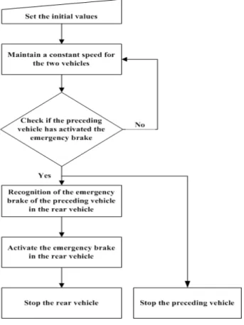
In this section we deal with the virtual operational scenario for the test of the proposed control scheme. Fig. 2 shows the task flow on the virtual control algorithm. In Fig.
2 the initial values for the parameters should be set to cal- culate the speed patterns of the both vehicles. The both vehicles are assumed that if there is no any activation for the emergency brake the both vehicles run on the guideway at a constant speed. However once the preceeding vehicle ac- tivates the emergency brake the rear vehicle should activate its emergency brake as soon as it recognizes the activation of the emergency brake in the preceeding vehicle.
3. Simulations
For simulations we employ a combined system which has Fig. 2. Task flow for the test algorithm
Fig. 3. Simulation model
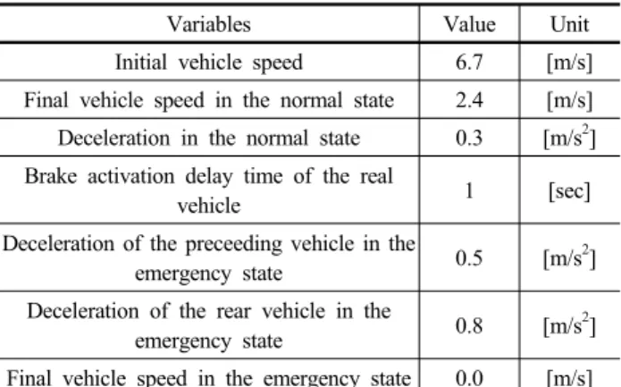
Matlab/Simulink and Labview Simulation Interface Toolkit to simulate the virtual operational scenario. Fig. 3 shows the simulation model which runs on the Matlab/Simulink plat- form. In the figure the preceeding vehicle speed pattern and the Rear vehicle speed pattern blocks calculate the braking curve of each vehicle based on the parameter information transferred from the Initial set block. For the monitoring of the braking curve we utilize Labview Simulation Interface Toolkit. Fig. 4 represents the front panel of Labview in- cluding the parameter initial values, speed pattern for normal state and speed pattern for emergency state.For the simula- tions we set the initial parameter values as shown in Table 1. It should be noted that the vehicle control commands which means the deceleration of the preceeding and rear vehicle in the emergency state are not the same. The reason is that it is necessary to stop the rear vehicle before the preceeding vehicle stops in order to avoid the collision between the vehicles in the emergency state. However in the real situations since each vehicle has the same brake per- formance it is necessary to employ MBS (Moving Block Sy- stem) control algorithm to avoid the collision between vehicles.
In this paper we assume that the vehicle control command can be input by manual for the test of the proposed control scheme.
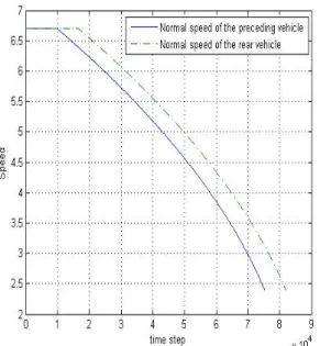
Fig. 5 and Fig. 6 show the simulation results. Fig. 5 is for the case of normal state. In this figure we see 1[sec] time delay in the rear vehicle to activate the brake, which means 6.7[m] in distance, due to the time duration to recognize the emergency brake activation in the preceeding vehicle. But both vehicles reach the same final vehicle speed, 2.4[m].
with 1[sec] time difference. It is because the vehicle control
Table 1. Initial parameters to calculate braking curve
Variables Value Unit
Initial vehicle speed 6.7 [m/s]
Final vehicle speed in the normal state 2.4 [m/s]
Deceleration in the normal state 0.3 [m/s2] Brake activation delay time of the real
vehicle 1 [sec]
Deceleration of the preceeding vehicle in the
emergency state 0.5 [m/s2]
Deceleration of the rear vehicle in the
emergency state 0.8 [m/s2]
Final vehicle speed in the emergency state 0.0 [m/s]
Fig. 4. Labview front panel
Fig. 5. Brake curve for the normal state
Fig. 6. Brake curve for the emergency state
command has set 0.3[m/s2] in both vehicles. In Fig. 6 speed patterns for the emergency states are shown. The rear vehicle activates its brake with 1[sec] time delay in comparison with the activation of the preceeding vehicle. However the rear vehicle stops with some safe distance before the preceeding vehicle dose.
4. Hardware Configurations
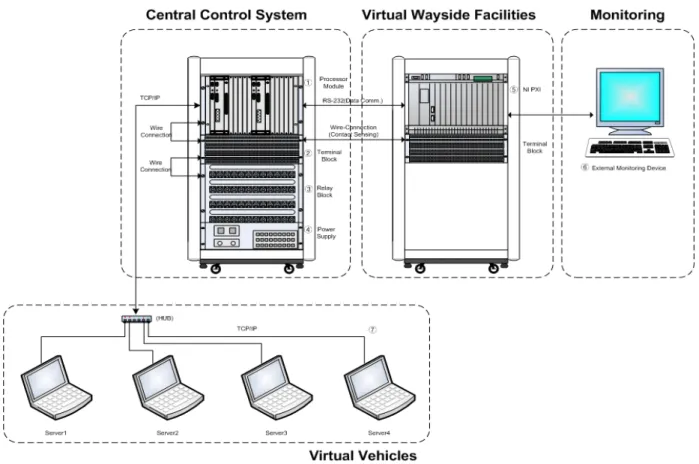
In this section, we deal with the hardware configuration of the proposed control scheme which is composed of virtual vehicles, central control system, virtual wayside facilities and monitoring device as shown in Fig. 7. The virtual vehicles can be implemented by using the several laptop computers which has the programed functions producing and displaying the vehicle status information. The number of the laptop computers can be arbitrary decided based on the system design. The central control system collects the information on each vehicle including the vehicle operational status and speed, and sends the parameter information to each vehicle
for the calculation of the braking curve in the on-board vehicle computer. In this paper, we employ MPC7410 microprocessor based VME bus processor module of Motorola Inc. including RS-232 ports, ethernet ports and VMEVMI2536 I/O board. The ethernet ports are used to transfer the vehicle status information and the vehicle control information between the central control system and the virtual vehicles. The calculated results are transferred to the virtual wayside facilities that can be implemented using the PXI module of the National Instruments Corporation, by way of the RS-232 ports, I/O board and the relay block. The role of the virtual wayside facilities is to display the current status of each vehicle based on the information transferred from the central control system. The monitoring device is installed to check the status of the central control system, virtual wayside facilities and the
virtual vehicles. It should be noted that we assumed there is no communication between the virtual vehicles to calculate the braking curve using the on-board vehicle computer in the proposed control scheme.
Fig. 7. Simple configuration of the proposed evaluation system
5. Experimental Results
Fig. 8 and 9 show the calculated results for the braking curve on VxWorks. As we see in the figures the experi- mental results have the same braking curves with the si- mulation results. This means that the proposed hardware configuration is valid and the communication protocol to make the interface between the virtual vehicles and the central control computer is established correctly.
6. Conclusions
In this paper we showed the quadratic equation to calculate the braking curve of the each vehicle and provided the simple operational scenario for the test of the simple control algorithm which has been simulated in the combined environment of Matlab/Simulink with Labview Simulation Interface Toolkit. The experimental results showed that the operational scenario for test worked very well in the proposed hardware configuration.
For future work it is necessary to create a elaborated ope- rational scenario which includes the acceleration, decelera- tion, stop, speed transition in main guideway, collision av- oidance between the vehicles.
References
1. Ollie Mikosza, Wayne D. Cottrell, “MISTER and other New- Generation Personal Rapid Transit Technology”, Transportation Research Board, 2007.
2. Jun-Ho Lee, Ducko Shin, Yong-Kyu Kim, “A Study on the Headway of the Personal Rapid Transit System”, Journal of the Korean Society for the Railway, Vol. 8, No. 6, pp.586-591, 2005.
3. Jun-Ho Lee, Kyung-Ho Shin, Jea-Ho Lee, Yong-Kyu Kim, “A Study on the Construction of a Control System for the Ev- aluation of the Speed Tracking Performance of the Personal Rapid Transit System”, Journal of the Korean Society for the Railway, Vol. 9, No. 4, pp.449-454, 2006.
4. Markus Theodor Szillat, “A Low-level PRT Microsimulation”, Ph. D. dissertation, University of Bristol, April 2001.
5. Duncan Mackinnon, “High Capacity Personal Rapid Transit System Developments”, IEEE Transactions on Vehicular Te- chnology, Vol. VT-24, No. 1, pp.8-14, 1975.
6. J.E. Anderson, “Control of Personal Rapid Transit”, Telektronikk 1, 2003.
7. Bih-Yuan Ku, Jyh-Shing R. Jang, Shang-Lin Ho, “A modulized Train Performance Simulator for Rapid Transit DC Analysis”, Proceedings of the 2000 ASME/IEE Joint Railroad Conference, pp.213-219, April, 2000.
년 월 일 논문접수 년 월 일 심사완료
(2007 6 1 , 2007 6 22 )
Fig. 9. Calculated results on VxWorks (emergency speed) Fig. 8. Calculated results on VxWorks (normal speed)