Measuring COVID-19 Effects on World and National Stock Market Returns

Print ISSN: 2288-4637 / Online ISSN 2288-4645 doi:10.13106/jafeb.2021.vol8.no2.0001

Measuring COVID-19 Effects on World and National Stock Market Returns*

Anya KHANTHAVIT ¹

Received: November 05, 2020 Revised: December 30, 2020 Accepted: January 08, 2021

Abstract

Previous studies have found the significant adverse effects of coronavirus disease 2019 (COVID-19) on stock returns and volatility. The effects varied with the confirmed cases and deaths. However, the extent of the effects have never been measured exactly. This study proposes a measurement model for the COVID-19 effects. In the proposed model, stock returns in the COVID-19 period are weighted averages of pre- COVID-19 normal returns and COVID-19-induced returns. The effects are measured by the contributing weights of the COVID-19-induced returns. Kalman filtering is used to estimate the model for the world and Chinese markets, in combination with 10 markets – five most affected countries (United States, India, Brazil, Russia, and France) and five best recovering countries (Hong Kong, Australia, Singapore, Thailand, and South Korea). The sample returns are daily, obtained from the closing Morgan Stanley global investable market indexes. The full period is from September 24, 2018, to October 30, 2020, whereas the COVID-19 period is from November 18, 2019, to October 30, 2020. The contributing weights are significant and close to 100% for all markets. The COVID-19-induced returns replace the pre-COVID-19 normal returns; they are negatively auto-correlated and highly volatile. The COVID-19-induced returns are new normal returns in the COVID-19 period.

Keywords: Kalman Filtering, New Normal, Pandemic, Return Behavior JEL Classification Code: G12, G14, G15

In addition to health disasters, COVID-19 has led to global economic and financial crises. The pandemic causes simultaneous worldwide disruptions to both supply–due to reduced labor supply and productivity, as well as lockdowns, business closures, and social distancing–and demand due to layoffs, loss of income, reduced household consumption, and declining firms’ investment (Chudik, Mohaddes, Pesaran, Raissi, & Rebucci, 2020). In January 2020, the World Bank (2020a) forecast the world’s real gross domestic product growth of 2.5% for 2020. In June 2020, after COVID-19 had spread, the organization revised the forecast downward to -5.2% (World Bank, 2020b). The spread of the disease continues, and the number of infected and death cases continues to increase. Economic problems persist and their future remains uncertain, leading to firms’ low expected cash flows and rising real and perceived risks. Consequently, stock prices drop (Harvey, 1989).

Despite extensive studies conducted on COVID-19 effects on stock market returns, none have addressed the extent of these effects and how stock returns changed from the pre-COVID-19 to COVID-19 periods. They showed either statistically significant abnormal returns due to the COVID-19 events or significant relationships of confirmed cases and deaths with returns and volatility.

*Acknowledgements:

*

The author thanks the Faculty of Commerce and Accountancy, Thammasat University, for the research grant, the Stock Exchange of Thailand for stock-index data, and Chanya Siriarayaphan for research assistance.

1

First Author and Corresponding Author. Distinguished Professor of Finance and Banking, Faculty of Commerce and Accountancy, Thammasat University, Thailand [Postal Address: No. 2 Phra Chan Road, Phra Nakhon, Bangkok, 10200, Thailand]

Email: [email protected]

© Copyright: The Author(s)

This is an Open Access article distributed under the terms of the Creative Commons Attribution Non-Commercial License (https://creativecommons.org/licenses/by-nc/4.0/) which permits unrestricted non-commercial use, distribution, and reproduction in any medium, provided the original work is properly cited.

1. Introduction

Coronavirus disease 2019 (COVID-19) is an infectious

respiratory disease caused by severe acute respiratory

syndrome coronavirus 2 (Lai, Shih, Ko, Tang, & Hsueh,

2020). The virus was first detected in Wuhan, China, on

November 17, 2019. Since October 30, 2020, COVID-19

has spread to 216 countries and territories, with a total

of 45,382,161 confirmed cases and 1,187,029 deaths

(Worldometers, 2020).

It is important to measure the extent of the effects because statistical significance does not necessarily imply financial significance. The resulting stock return behavior in the COVID-19 period has practical implications for asset allocation (Song, Siu, Ching, Tong, & Yang, 2012), risk measurement (Duffie & Pan, 1997), stock trading (Diether, Lee, & Werner, 2009), and derivative pricing (Bates, 2003).

This study proposes a model to measure the COVID-19 effects on stock returns. The stock return during the COVID-19 sample is a weighted average of the pre- COVID-19 normal returns and COVID-19-induced returns.

The study estimates the two returns and their contributing weights using Kalman filtering. The normal return is the return during the pre-COVID-19 sample. The COVID-19 effects are measured by the contributing weight of the COVID-19-induced return.

2. Literature Review

In international studies, Bash (2020), Khanthavit (2020a), and Liu, Manzoor, Wang, Zhang, and Manzoor (2020) reported negative and significant effects of COVID-19 on stock market returns. These effects were stronger with rising confirmed cases and deaths (Cao, Li, Liu, & Woo, 2020;

Khan et al., 2020). Significant positive abnormal returns were detected for some national markets during certain sub- periods. For example, for the Indian market, Alam, Alam, and Chavali (2020) reported significant, positive abnormal returns during the lockdown period, whereas significant, negative abnormal returns were observed during the pre- and post-lockdown periods. The market believed that the lockdown would stop the virus from spreading.

Within a certain market, COVID-19 affects stocks in different sectors or both in positive and negative ways.

For example, for the US market, Ramelli and Wagner (2020) found that stocks in the utility, healthcare, and telecommunication sectors were positively affected, whereas those in the transportation, automobile, and energy sectors were negatively affected. For the Chinese market, He, Sun, Zhang, and Li (2020) reported the positive effects of COVID-19 for stocks in the public management, information technology, and sports and entertainment sectors. Further, the effects for the stocks in the transportation, construction, environment, electric and heating, real estate, health, education, agriculture, and mining sectors were negative, whereas those for the stocks in the scientific research and lodging and catering sectors were marginal. It is interesting to learn that, in the US market, the negative effects on stocks with high environmental and social ratings were less severe (Albuquerque, Koskinen, Yang, & Zhang, 2020). Al-Awadhi, AlSaifi, Al-Awadhi, and Alhammadi (2020) found that, for the Chinese market, class-B stocks experienced significantly more negative effects than class-A stocks. Moreover, stocks

with larger market capitalization were affected more severely than those with smaller market capitalization.

COVID-19 also affects stock volatility. Baker, Bloom, Davis, Kost, Sammon, and Viratyosin (2020) linked increasing stock volatility with COVID-19 due to government limitations on commercial activities and restrictions on consumers. Zaremba, Kizys, Aharon, and Demir (2020) added that governments’ rigorous actions, such as information campaigns and cancellation of public events, to mitigate the spread of the disease heightened the volatility. The fact that COVID-19 can affect stock volatility is supported by Albulescu (2020) and Onali (2020). They found that stock volatility increased with the number of confirmed cases and deaths. In addition to its short-term effects, COVID-19 affects permanent stock volatility (Bai, Wei, Wei, Li, & Zhang, 2020).

3. Research Method and Data 3.1. The Model

Let _rt be the random stock return on day t. The study assumes that the stock return _rt moves normally during the pre-COVID-19 period. During the COVID-19 period, the disease causes the stock return to behave differently. The return is a weighted average of the pre-COVID-19 normal returns and COVID-19-induced returns. Equation (1) summarizes the return behavior in the pre-COVID-19 and COVID-19 periods.

, ..., 1 (1 )

0, ...,

tN

N C

t t

for t T

rt γ r r r for t

τ γ

 = − −

=    − + =

 

  , (1)

where r

t^N

and r

t^C

are the pre-COVID-19 normal and COVID-19-induced returns, respectively, and γ is the contributing weight of r

_t^C

to _rt . Moreover, Day t = 0 is the event day on which the market acknowledged the COVID-19 virus for the first time; hence, the periods from days t = − T to t = − 1 and t = 0 to t = τ are the pre-COVID-19 and COVID-19 periods, respectively.

The study decomposes the stock return r

_tⁱ

into the expected return µ _

tⁱ

and error term e

tⁱ

, where i = N, C indicates the pre-COVID-19 and COVID-19 variables.

i i i

t t t

r  = µ  + e  (2)

The error term e

tⁱ

has a zero mean and σ

eⁱ

standard deviation. The expected return µ _

_tⁱ

follows an autoregressive process of order 1 (AR(1)) in equation (3).

0 1 1

i i i i i

t t t

µ  = α + α µ

₋

+ ε  (3)

The parameter α

0i

is the intercept, whereas the parameter

1i

α is the slope, AR(1) coefficient. The error term ε _

tⁱ

has a zero mean and σ

_εⁱ

standard deviation, and the AR(1) specification is general. This is consistent with the return autocorrelation observed for stocks in various national markets (Khanthavit, 2020a). The model implies the mean- adjusted specification widely used in event study analyses (Brown & Warner, 1985), when α

₁ⁱ

= σ ε

ⁱ

= 0.

The model in equations (1), (2), and (3) is the modified model from Khanthavit (2020b). In that study, _rt is foreign investors’ trading volume, r 

_t^N

+ µ 

_t^C

is the return behavior in the COVID-19 period, and the µ _

_t^C

component is the abnormal return.

In this study, the different return behaviors during the COVID-19 period from the pre-COVID-19 period are not considered abnormal behaviors; thus, the COVID-19-induced return is not an abnormal return. The study recognizes Goodell (2020) in that COVID-19 presents a new normal to investors.

Therefore, stock returns during the COVID-19 period behave in a new normal way. The specification (1 − γ ) r 

t^N

+ γ r 

t^C

describes the new normal return.

3.2. Model Estimation

Combining equations (1) and (2) results in ,..., 1 {(1 ) } 0,..., .

{(1 ) }

tN tC

N C

t t

for t T

N for t

r t

e e

µ

γ µ γµ τ

γ γ

 + = − −

 − + + =

=    − +



 



 

(4)

Equations (3) and (4) constitute a state-space model for the stock returns during the pre-COVID-19 and COVID-19 periods. Equation (4) is the measurement equation in which the observed return is related to the unobserved expected returns µ _

_t^N

and µ _

_t^C

. Equation (3) is the transition equation that describes the stochastic behaviors of the unobserved state variables. Here, the state variables are the expected returns µ _

_t^N

and µ _

_t^C

. The transition equation (3) can be rewritten as a system of equations as in equation (5).

0 1

0 1 1

0 ,

0

N N N N N

t t t t

C C C C C

t t t

µ α α µ ε

µ α α µ

⁻₋

ε

         

= + +

         

 

       

  



  (5)

where the covariance matrix of

^tN_C

t

ε ε

 

 

 



 is ( )

²

0

₂

. 0 ( )

N C

ε

ε

σ σ

 

 

 

This study assumes the uncorrelated error terms ε _

_t^N

and ε _

t^C

. because, under the null hypothesis of no COVID-19 effects,

C

µ _

t

is zero. For the same reason, the error terms e

_t^N

and e

_t^C

are uncorrelated between each other and with ε _

_t^N

and ε _

t^C

. This study uses Kalman filtering to estimate the state-space model in equations (4) and (5) (Harvey, 1990).

3.3. Hypothesis Tests

3.3.1. Measuring the COVID-19 Effects

From equation (1), the contributing weight γ enables the study to precisely measure the COVID-19 effects. If the COVID-19 effects are temporary or non-existent,

γ is small because it is averaged out over time or zero initially. The hypothesis is γ = 0 . A significant γ indicates permanent COVID-10 effects and a new normal market.

However, if γ = 1, the new normal returns r r 

t

= 

t^C

. The COVID-19-induced return replaces the pre-COVID-19 normal return.

3.3.2. Difference Between Pre-COVID-19 Normal Return and COVID-19-Induced Return

Although is non-zero, a new normal market requires different processes for the pre-COVID-19 normal return and COVID-19-induced return. Under a non-difference hypothesis, at least one of the following hypotheses is rejected: α

₀^N

= α α

₀^C

,

₁^N

= α σ

₁^C

, _ε

^N

= σ _ε

^C

, and σ

_e^N

= σ

_e^C

. Each hypothesis is tested in this study. The joint hypothesis is also tested using a Wald test. Under the joint hypothesis, the Wald statistic is distributed as a chi-square variable with four degrees of freedom.

3.4. The Data

This study estimates the state-space model in equations (4) and (5) for stocks in the five most affected countries and five best recovering countries. On October 30, 2020, the most affected countries are the United States, India, Brazil, Russia, and France (Worldometers, 2020), whereas the best recovering countries are Hong Kong, Australia, Singapore, Thailand, and South Korea (PEMANDU Associates, 2020). The study also considers the world and Chinese stock markets. The world market serves as a representative of the national markets worldwide. Meanwhile, the Chinese market is important and interesting because the COVID-19 virus was first detected in China.

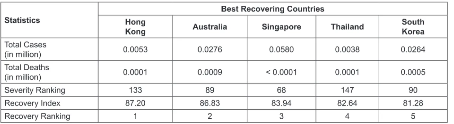
Table 1 reports the COVID-19 statistics for severity and recovery. Severity is measured by confirmed cases and deaths, whereas recovery is measured by the recovery indices of PEMANDU Associates. The United States contributed about a fifth to the world’s confirmed cases and deaths.

Although it is the first country that experienced the disease, China has managed the situation well. Its rankings in terms of severity and recovery are 56th and 10th, respectively.

In particular, the best market in terms of recovery is Hong

Kong, and it contributes only approximately 0.01% to the

world’s confirmed cases and deaths.

The sample returns are the daily logged returns scaled by 100. They are derived from closing Morgan Stanley global investable market indexes. The market indexes are in local currencies, and the world index is in US dollars. The indexes include large, medium, and small capitalization stocks, resulting in the inclusion of approximately 99% of the free float-adjusted market capitalization. They were retrieved from the Morgan Stanley database (www.msci.com/end-of-day-data-country).

To choose the sample period, day t = 0 must be identified. This study follows Khanthavit (2020a; 2020b) to fix day t = 0 for November 17, 2019. The day, November 17, 2020, is the first day that COVID-19 was detected in China (Mimouni et al., 2020). Because November 17, 2019, fell on a Sunday, day t = 0 is adjusted to Monday, November 18, 2019—the first trading day after November 17, 2019.

At the time of this study, COVID-19 continues to spread.

The last available sample return is for October 30, 2020;

thus, the COVID-19 sample covers a period from November 18, 2019, to October 30, 2020 (250 daily observations).

Next, the pre-COVID-19 sample was selected in this study, during which time the return behaved normally and was unaffected by COVID-19. In statistics, a long sample

period is preferred. However, Nazir, Younus, Kaleem, and Anwar (2014) cautioned that a long pre-COVID-19 sample absorbed the economic and noneconomic events irrelevant to the study. The typical lengths of the pre-event period range from 100 to 300 days (Peterson, 1989). With respect to Nazir et al. (2014) and Salinger (1992), the study chooses the longest period of 300 days for accurate parameter estimation.

The pre-COVID-19 sample begins on September 24, 2018, and ends November 15, 2019, resulting in the full sample ranging from September 24, 2018, to October 30, 2020 (550 daily observations).

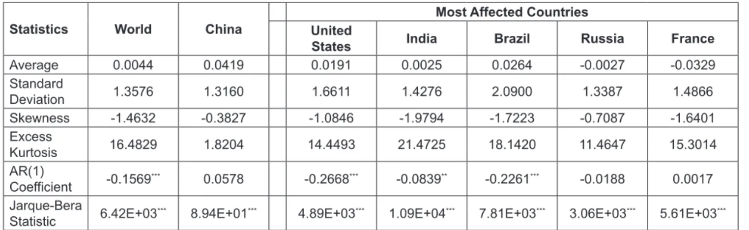
Table 2 reports the descriptive statistics of the sample returns. In Panel 2.1, the full-sample returns for all the markets are negatively skewed and fat-tailed. The AR(1) coefficients are negative and significant for most markets.

The Jarque–Bera statistics reject the normality hypothesis for all the markets. The AR(1) specification for returns in equation (3) is supported by significant autocorrelation.

Although the Jarque–Bera statistics reject the normality hypothesis for the returns in all markets, Kalman filtering can still be used. The filter is optimal and produces the minimum mean square linear estimates (Kellerhals, 2001).

Table 1: COVID-19 Severity and Recovery Statistics

Statistics World China Most Affected Countries

United

States India Brazil Russia France

Total Cases

(in million) 45.3821 0.0859 9.2128 8.0889 5.4964 1.6000 1.2828

Total Deaths

(in million) 1.1870 0.0046 0.2342 0.1211 0.1590 0.0277 0.0360

Severity Ranking N.A. 56 1 2 3 4 5

Recovery Index N.A. 75.40 42.67 65.00 62.31 57.14 28.58

Recovery Ranking N.A. 10 138 27 41 65 166

N.A. denotes non-applicable.

Table 1: COVID-19 Severity and Recovery Statistics (Continued)

Statistics Best Recovering Countries

Hong Kong Australia Singapore Thailand South

Korea Total Cases

(in million) 0.0053 0.0276 0.0580 0.0038 0.0264

Total Deaths

(in million) 0.0001 0.0009 < 0.0001 0.0001 0.0005

Severity Ranking 133 89 68 147 90

Recovery Index 87.20 86.83 83.94 82.64 81.28

Recovery Ranking 1 2 3 4 5

Table 2 reports the descriptive statistics of the sample returns. In Panel 2.1, the full-sample returns for all the markets are negatively skewed and fat-tailed. The AR(1) coefficients are negative and significant for most markets. The Jarque–Bera statistics reject the normality hypothesis for all the markets. The AR(1) specification for returns in equation (3) is supported by significant autocorrelation. Although the Jarque–Bera statistics reject the normality hypothesis for the returns in all markets, Kalman filtering can still be used. The filter is optimal and produces the minimum mean square linear estimates (Kellerhals, 2001).

Panels 2.2 and 2.3 report the statistics for the pre- COVID-19 and COVID-19 samples, respectively. With respect to the AR(1) coefficients, the negative, significant AR(1) coefficients for the full sample result from the AR(1) coefficients in the COVID-19 sample. The normality hypothesis is rejected by the Jarque–Bera statistics for all the

markets for the two samples, except for the Russian market for the pre-COVID-19 sample.

Lyócsa, Baumöhl, Výrost, and Molnár (2020) observed that COVID-19 brought unprecedented declines and high uncertainty in the global stock markets. This study tests for the equal means and standard deviations for the returns in the pre-COVID-19 and COVID-19 samples. As shown in Panel 2.4, the mean returns are larger for the pre-COVID-19 samples than for the COVID-19 samples for the world, Brazilian, Russian, French, Hong Kong, Australian, Singaporean, and Thai markets, whereas those for the remaining markets are smaller. Thus, the equal mean return hypothesis cannot be rejected for any market. The test for equal standard deviations rejects the null hypothesis for all markets. This finding supports high uncertainty, but not falling markets.

It also suggests that the falling markets observed by Lyócsa et al. (2020) are for short term. In particular, the markets recovered in the later period of the COVID-19 sample.

Table 2: Descriptive Statistics

Panel 2.1: Full Sample from September 24, 2018, to October 30, 2020 (550 observations)

Statistics World China Most Affected Countries

United

States India Brazil Russia France

Average 0.0044 0.0419 0.0191 0.0025 0.0264 -0.0027 -0.0329

Standard

Deviation 1.3576 1.3160 1.6611 1.4276 2.0900 1.3387 1.4866

Skewness -1.4632 -0.3827 -1.0846 -1.9794 -1.7223 -0.7087 -1.6401

Excess

Kurtosis 16.4829 1.8204 14.4493 21.4725 18.1420 11.4647 15.3014

AR(1)

Coefficient -0.1569

^***

0.0578 -0.2668

^***

-0.0839

^**

-0.2261

^***

-0.0188 0.0017 Jarque-Bera

Statistic 6.42E+03

^***

8.94E+01

^***

4.89E+03

^***

1.09E+04

^***

7.81E+03

^***

3.06E+03

^***

5.61E+03

^***

**

and

^***

denote significance at the 95% and 99% confidence levels, respectively.

Panel 2.1: Full Sample from September 24, 2018, to October 30, 2020 (550 observations) (Continued)

Statistics Best Recovering Countries

Hong Kong Australia Singapore Thailand South

Korea

Average -0.0232 -0.0095 -0.0433 -0.0854 0.0013

Standard Deviation 1.2764 1.4119 1.1190 1.3829 1.3793

Skewness -0.5272 -1.4016 -0.6139 -2.0712 -0.1274

Excess Kurtosis 3.8560 12.2001 12.0013 21.9750 8.2501

AR(1) Coefficient -0.0031 -0.2357

^***

-0.0303 -0.1429

^***

-0.0450

Jarque-Bera Statistic 3.66E+02

^***

3.59E+03

^***

3.34E+03

^***

1.15E+04

^***

1.56E+03

^***

***

denote significance at the 99% confidence level.

Panel 2.2: Pre-COVID-19 Sample from September 24, 2018, to November 15, 2019 (300 observations)

Statistics World China Most Affected Countries

United

States India Brazil Russia France

Average 0.0123 -0.0107 0.0171 -0.0021 0.0904 0.0639 0.0207

Standard

Deviation 0.7809 1.1668 1.0014 0.9089 1.2045 0.8789 0.8983

Skewness -0.4493 -0.1168 -0.3052 0.3981 -0.0089 0.0565 -0.5430

Excess

Kurtosis 1.8199 0.5884 3.1322 2.7001 0.9986 0.2818 1.5561

AR(1)

Coefficient 0.1615

^***

0.1526

^***

0.0327 0.0745 -0.0199 -0.0294 0.0552

Jarque-Bera

Statistic 51.4945

^***

5.0106

^*

1.27E+02

^***

99.0553

^***

12.4700

^***

1.1517 45.0139

^***

*

and

^***

denote significance at the 90% and 99% confidence levels, respectively.

Panel 2.2: Pre-COVID-19 Sample from September 24, 2018, to November 15, 2019 (300 observations) (Continued)

Statistics Best Recovering Countries

Hong Kong Australia Singapore Thailand South

Korea

Average -0.0159 0.0292 0.0107 -0.0441 -0.0203

Standard Deviation 1.0821 0.7451 0.6561 0.7255 0.9323

Skewness 0.1164 -0.8766 -0.4173 -0.1149 -0.4677

Excess Kurtosis 2.3282 2.3541 2.2311 1.3124 2.6650

AR(1) Coefficient 0.0458 0.0396 0.0388 -0.0555 -0.0106

Jarque-Bera Statistic 68.4340

^***

1.08E+02

^***

70.9288

^***

22.1912

^***

99.7154

^***

***

denote significance at the 99% confidence level.

Panel 2.3: COVID-19 Sample from November 18, 2019, to October 30, 2020 (250 observations)

Statistics World China Most Affected Countries

United

States India Brazil Russia France

Average -0.0052 0.1050 0.0214 0.0079 -0.0504 -0.0827 0.0214

Standard

Deviation 1.8252 1.4752 2.2089 1.8712 2.8067 1.7355 2.2089

Skewness -1.2783 -0.5806 -0.9897 -2.0082 -1.5064 -0.6255 -0.9897

Excess

Kurtosis 10.0754 2.1733 9.1317 15.1390 11.1587 8.0200 9.1317

AR(1)

Coefficient -0.2269

^***

-0.0166 -0.3408

^***

-0.1285

^**

-0.2732

^***

-0.0187 -0.3408

^***

Jarque-Bera

Statistic 1.13E+03

^***

63.2437

^***

9.09E+02

^***

2.56E+03

^***

1.39E+03

^***

6.86E+02

^***

9.09E+02

^***

**

and

^***

denote significance at the 95% and 99% confidence levels, respectively.

Panel 2.3: COVID-19 Sample from November 18, 2019, to October 30, 2020 (250 observations) (Continued)

Statistics Best Recovering Countries

Hong Kong Australia Singapore Thailand South

Korea

Average -0.0972 -0.0321 -0.0560 -0.1081 -0.1349

Standard Deviation 1.9738 1.4785 1.9299 1.4954 1.8921

Skewness -1.4120 -0.7976 -1.0926 -0.4214 -1.7156

Excess Kurtosis 9.7059 3.6176 6.4510 7.1665 12.5968

AR(1) Coefficient -0.0135 -0.0351 -0.2858

^***

-0.0500 -0.1597

^**

Jarque-Bera Statistic 1.06E+03

^***

1.63E+02

^***

4.83E+02

^***

5.42E+02

^***

1.78E+03

^***

**

and

^***

denote significance at the 95% and 99% confidence levels, respectively.

Panel 2.4: Tests for Equal Means and Standard Deviations in the Pre-COVID-19 and COVID-19 Samples

Statistics World China Most Affected Countries

United

States India Brazil Russia France

Mean

Difference 0.0175 -0.1158 -0.0043 -0.0100 0.1409 0.1466 0.1179

Standard- Deviation

Difference -1.0443

^***

-0.3083

^***

-1.2074

^***

-0.9622

^***

-1.6022

^***

-0.8566

^***

-1.0755

^***

***

denotes significance at the 99% confidence level.

Panel 2.4: Tests for Equal Means and Standard Deviations in the Pre-COVID-19 and COVID-19 Samples (Continued)

Statistics Best Recovering Countries

Hong Kong Australia Singapore Thailand South

Korea

Mean Difference 0.0162 0.0853 0.1188 0.0908 -0.0475

Standard-Deviation

Difference -0.3964

^***

-1.1848

^***

-0.8394

^***

-1.1666

^***

-0.8424

^***

***

denotes significance at the 99% confidence level.

4. Empirical Results 4.1. Parameter Estimates

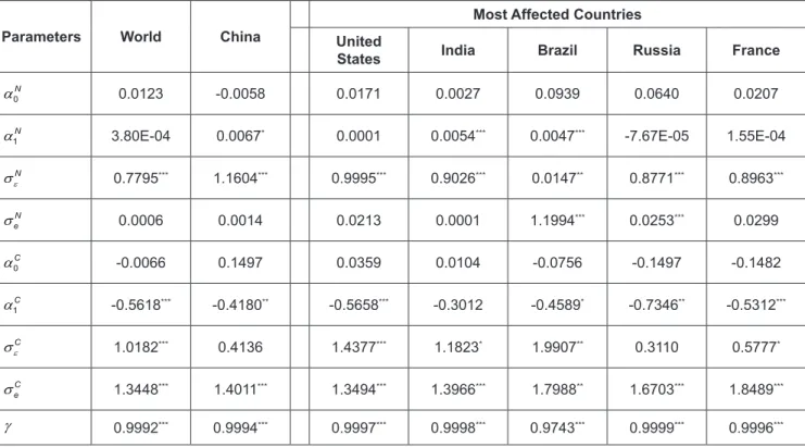
The parameter estimates are reported in Panel 3.1 of Table 3. The intercepts α

₀^N

and α

₀^C

for the pre-COVID-19 normal and COVID-19-induced returns, respectively, are non-significant. This result supports the small mean returns and non-significant mean difference reported in Table 2. The results for the slope coefficients α

₁^N

for the normal returns are mixed. They are significant and positive for China, India, Brazil, and Hong Kong. The remaining variables are non-significant. Hence, the negative AR(1) coefficients

in Panel 2.3, Table 2, are explained by the negative slope coefficients α

₁^C

for the COVID-19-induced returns. The large standard deviations found for the sample stocks in the COVID-19 sample are explained further by the error terms

tC

e of random returns r

t^C

than by the error terms ε 

t^C

of

random expected returns µ _

_t^C

. The exceptions are the United

States, Brazilian, Australian, and Thai markets, with reverse

case. Finally, the contributing weights γ are significant

at the 99% confidence level for all markets. The largest

effects are for the Russian market (i.e., 99.99%), whereas

the smallest effects are for the Brazilian market (i.e.,

97.43%). The study concludes that the COVID-19 effects

are significant and very large.

4.2. Hypothesis Tests

4.2.1. COVID-19-Induced Returns Replace Normal Returns

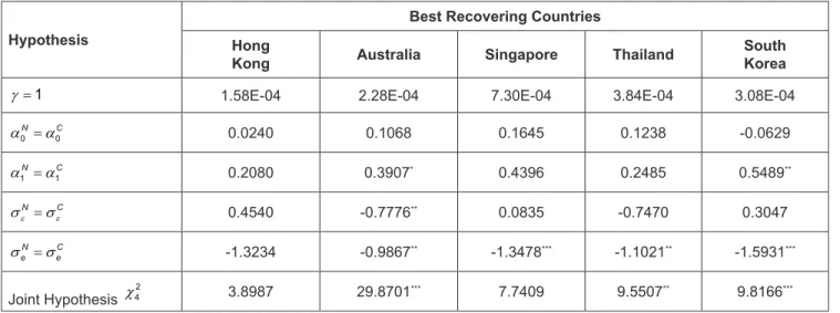
The hypothesis whether COVID-19-induced returns replace the pre-COVID-19 normal returns is tested in this study. Under the null hypothesis, γ = 1 and r r

_t

=

_t^C

during the COVID-19 period. In row 2 of Panel 3.2, Table 3, the hypothesis cannot be rejected for any market, except for the Brazilian market. For the Brazilian market, the significant difference of γ from is 2.57%; the contribution of the normal return r

t^N

during the COVID-19 period is small. The finding that γ = 1 is consistent with that of Onali (2020), who found from a Markov-switching test for Dow-Jones returns that the probability of returns being in the COVID-19 state was greater than 0.99.

4.2.2. Different Processes for Pre-COVID-19 Normal and COVID-19-Induced Returns

Although the contributing weights γ of COVID-19- induced returns are large and significant for all the sample

markets, the new normal returns are essentially the same as the normal returns if the parameters ( , α α σ σ

₀^N ₁^N

, ε

^N

,

_e^N

) and

0 1

( , α α σ σ

^{C C}

, _ε

^C

,

_e^C

) are not significantly different. This study conducted a joint hypothesis test for equal parameters. The results are reported in the last row of Panel 3.2, Table 3.

The Wald test rejects the hypothesis for all countries, except for India, Hong Kong, and Singapore. However, when the study conducts separate tests for parameter pairs—

0^N 0^C

,

1^N 1^C

, ε

^C

ε

^N

,

α = α α = α σ = σ and σ

_e^C

= σ

_e^N

, the results show that the hypothesis σ

_e^C

= σ

_e^N

is rejected for the Indian and Singaporean markets. Conversely, none of the four hypotheses is rejected for the Hong Kong market.

The study examines why the results for Hong Kong are non-significant. From Panel 2.4, Table 2, the standard deviations of returns in the COVID-19 sample are significantly larger than those in the pre-COVID-19 sample. Based on this finding, the study examines the sizes of σ σ ε

^N

( )

_e^C

vis-à-vis σ σ ε

^N

( )

_e^C

from Panel 3.1, Table 3. The sizes are σ _ε

^N

= 1.7086 ( σ

_e^C

= 0.6243) and

0.0073 ( 1.3307).

N C

e

σ ε = σ = The parameters σ ε

^N

and σ

e^C

are significant, and the sizes of the parameters in each pair are financially different. It is likely that non-significance for Hong Kong results from imprecise estimates σ

_e^N

and σ _ε

^C

.

Table 3: Parameter Estimates and Hypothesis Tests Panel 3.1: Parameter Estimates

Parameters World China

Most Affected Countries United

States India Brazil Russia France

α

₀^N

0.0123 -0.0058 0.0171 0.0027 0.0939 0.0640 0.0207

α

₁^N

3.80E-04 0.0067

^*

0.0001 0.0054

^***

0.0047

^***

-7.67E-05 1.55E-04

σ

ε^N

_0.7795

^***

_1.1604

^***

_0.9995

^***

_0.9026

^***

_0.0147

^**

_0.8771

^***

_0.8963

^***

σ

_e^N

_{0.0006 0.0014 0.0213 0.0001 1.1994}

^***

_0.0253

^***

_0.0299

α

₀^C

_{-0.0066 0.1497 0.0359 0.0104 -0.0756 -0.1497 -0.1482}

α

₁^C

_-0.5618

^***

_-0.4180

^**

_-0.5658

^***

_{-0.3012 -0.4589}

^*

_-0.7346

^**

_-0.5312

^***

σ

ε^C

1.0182

^***

0.4136 1.4377

^***

1.1823

^*

1.9907

^**

0.3110 0.5777

^*

σ

^C_e

1.3448

^***

1.4011

^***

1.3494

^***

1.3966

^***

1.7988

^**

1.6703

^***

1.8489

^***

γ _0.9992

^***

_0.9994

^***

_0.9997

^***

_0.9998

^***

_0.9743

^***

_0.9999

^***

_0.9996

^***

*

,

^**

, and

^***

denote the significance at the 90%, 95%, and 99% confidence levels, respectively.

Panel 3.2: Hypothesis Tests

Hypothesis World China

Most Affected Countries United

States India Brazil Russia France

γ = 1 8.22E-04 6.50E-04 2.79E-04 1.66E-04 0.0257

^***

5.16E-05 3.68E-04

α

₀^N

= α

₀^C

0.0189 -0.1555 -0.0188 -0.0077 0.1695 0.2136 0.1689

α

₁^N

= α

₁^C

0.5622

^***

0.4246

^**

0.5660

^***

0.3066 0.4636

^*

0.7345

^**

0.5313

^***

ε ε

σ

^N

= σ

^C

-0.2387 0.7468

^**

-0.4381 -0.2797 -1.9760

^**

0.5661

^**

0.3186

σ

_e^N

= σ

^C_e

-1.3442

^***

-1.3997

^***

-1.3281

^***

-1.3965

^***

-0.5994 -1.6449

^**

-1.8190 Joint

Hypothesis

χ

₄²

^18.7597

***

42.6904

^***

27.1743

^***

3.0281 67.0403

^***

44.0934

^***

13.1395

^***

*

,

^**

, and

^***

denote the significance at the 90%, 95%, and 99% confidence levels, respectively.

Panel 3.1: Parameter Estimates (Continued) Parameters

Best Recovering Countries

Hong Kong Australia Singapore Thailand South

Korea

α

₀^N

-0.0135 0.0292 0.0107 -0.0441 -0.0203

α

₁^N

0.0033

^***

6.72E-05 5.00E-05 -1.25E-04 -2.75E-05

σ

ε^N

1.0786

^***

0.7438

^***

0.6550

^***

0.7240

^***

0.9307

^***

σ

_e^N

_{0.0073 0.0020}

^***

_{0.0035 0.0209 0.0127}

α

₀^C

_{-0.0375 -0.0776 -0.1537 -0.1680 0.0427}

α

₁^C

_{-0.2046 -0.3907}

^*

_{-0.4396 -0.2486 -0.5489}

^**

σ

ε^C

_{0.6246 1.5214}

^***

_{0.5714 1.4710}

^*

_0.6259

σ

^C_e

1.3307

^***

0.9888

^**

1.3513

^***

1.1230 1.6058

^***

γ _0.9998

^***

_0.9998

^***

_0.9993

^***

_0.9996

^***

_0.9997

^***

*

,

^**

, and

^***

denote the significance at the 90%, 95%, and 99% confidence levels, respectively.

Table 4: Checks for Robustness and Early Effects

Parameters World China Most Affected Countries

United

States India Brazil Russia France

γ

₁

_0.9930

^***

_0.9997

^***

_0.9936

^***

_0.9975

^***

_0.9920

^***

_0.9999

^***

_0.9999

^***

γ

₂

_0.9996

^***

_0.9996

^***

_0.9999

^***

_0.9999

^***

_0.9999

^***

_0.9999

^***

_0.9998

^***

γ

₂

− γ 4.71E-04 1.87E-04 1.36E-04 8.09E-05 0.0257

^***

2.74E-05 1.67E-04

* and *** denote the significance at the 90% and 99% confidence levels, respectively. The estimates γ and γ

₁

are for the cases in which days t = 0 are November 18, 2019, and January 20, 2020, respectively, whereas the estimate γ

₂

is for a shorter COVID-19 sample from November 18, 2019, to March 31, 2020. The full parameter estimates can be obtained from the author upon request.

Table 4: Checks for Robustness and Early Effects (Continued)

Parameters Best Recovering Countries

Hong Kong Australia Singapore Thailand South

Korea

γ

₁

_0.9461

^***

_0.9946

^***

_0.9973

^***

_0.9999

^***

_0.9980

^***

γ

₂

_0.9996

^***

_0.9999

^***

_0.9998

^***

_0.9999

^***

_0.9999

^***

γ

₂

− γ -2.47E-04 1.90E-04

^*

5.01E-04 2.02E-04 2.21E-04

* and *** denote the significance at the 90% and 99% confidence levels, respectively. The estimates γ and γ

₁

are for the cases in which days t = 0 are November 18, 2019, and January 20, 2020, respectively, whereas the estimate γ

₂

is for a shorter COVID-19 sample from November 18, 2019, to March 31, 2020. The full parameter estimates can be obtained from the author upon request.

Panel 3.2: Hypothesis Tests (Continued) Hypothesis

Best Recovering Countries

Hong Kong Australia Singapore Thailand South

Korea

γ = 1 1.58E-04 2.28E-04 7.30E-04 3.84E-04 3.08E-04

α

₀^N

= α

₀^C

0.0240 0.1068 0.1645 0.1238 -0.0629

α

₁^N

= α

₁^C

0.2080 0.3907

^*

0.4396 0.2485 0.5489

^**

ε ε

σ

^N

= σ

^C

0.4540 -0.7776

^**

0.0835 -0.7470 0.3047

σ

_e^N

= σ

^C_e

-1.3234 -0.9867

^**

-1.3478

^***

-1.1021

^**

-1.5931

^***

Joint Hypothesis χ

₄²

_{3.8987 29.8701}

^***

_{7.7409 9.5507}

^**

_9.8166

^***

*

,

^**

, and

^***

denote the significance at the 90%, 95%, and 99% confidence levels, respectively.

5. Discussion

5.1. Alternative Choices for the First Day of the COVID-19 Period

In previous studies, researchers proposed alternative choices for the days that the COVID-19 period began.

The study checked for robustness of results due to these alternative choices. The state-space model is re-estimated for the sample countries, when Day t = 0 is January 20, 2020, on which day human-to-human transmission of COVID-19 was confirmed. This alternative was chosen by Liu et al. (2020).

This study is based on Liu et al.’ (2020) study because the discovery of human-to-human transmission is an important event. The day January 20, 2020, is also the day the United States experienced the first COVID-19 case, and the abnormal Google search volume on COVID-19 was first detected (Kapar, Buigut, & Rana, 2020). The date is close to January 23, 2020, on which China quarantined Wuhan to stop the spread of the disease. The day January 23, 2020, was chosen by He et al. (2020) as the first day of the COVID-19 period.

This study did not consider December 30, 2019, when China informed the World Health Organization (WHO) of patients with mysterious pneumonia (Cheema, Faff, &

Szulczuk, 2020) because the date is close to November 17, 2019. It did not choose the days the disease became known to the media because those days are country-dependent (Kim, Kim, Lee, & Tang, 2020).

The results for January 20, 2020, as the first day of the COVID-19 period is reported in the second row of Table 4. Only the contributing weights γ

₁

are shown, and all the weights are significant at the 99% confidence level.

The large sizes are greater than 99%, except for the Hong Kong market. It is noted that the weights for January 20, 2020, are smaller than those for November 17, 2019, and the exceptions are the Chinese, Brazilian, French, and Thai markets.

5.2. Early Effects

Topcu and Gulal (2020) studied the effects of COVID-19 on emerging stock markets in South America, the Middle East, Europe, and Asia. By considering the effects for sub- samples, the researchers found that the effects were stronger in the early sub-sample and began to taper off in the later sub-sample. This study examines the stronger effects of COVID-19 during the early period of its spread. Following Topcu and Gulal (2020), it limits the full sample to a period from September 24, 2018, to March 31, 2020. The resulting weights γ

₂

are reported in row 3 of Table 4. If the effects are stronger in the early period, γ

₂

> γ , where γ is the

contributing weight for the sample from September 24, 2018, to October 30, 2020. The test for hypothesis γ

₂

= γ is reported in row 4.

The study found that γ

₂

is very large for all the sample markets, and they are significant at the 99% confidence level. Although they are larger than γ , the difference is not significant. This finding is consistent with that of Topcu and Gulal (2020). The non-significant result can be explained by the fact that the effects in the later period are also very large and that the estimation of γ

₂

includes the early period in the COVID-19 sample.

The strong market reaction in the early COVID-19 period explains the weak effects for the (January 20, 2020) specification reported in the previous sub-section. The estimation does not include the early sample from November 18, 2019, to January 19, 2020, in the COVID-19 sample. The excluded sample is the period of the disease’s early spread.

5.3. Over-Reaction

Phan and Narayan (2020) studied stock returns in 25 markets in most affected countries and found an over- reaction behavior. The researchers explained over-reaction by the markets’ response to unexpected information on COVID-19. Thereafter, the markets corrected themselves as more information was available. In this study, the significant, negative AR(1) coefficients in Panels 2.1 and 2.3, Table 2, suggests the over-reaction behavior of the sample stocks in the COVID-19 sample. Panel 3.1, Table 3, offers an insightful explanation. The parameters are negative and significant; thus, over-reaction is attributed to the COVID- 19-induced returns.

5.4. COVID-19-Induced Volatility

In Table 2, stock volatility increased substantially during the COVID-19 period compared to the pre-COVID-19 period. This finding is consistent with Albulescu (2020) and Onali (2020). From the return structure in equations (4) and (5), when the contributing weights γ for all the markets are close to 1.00, large sizes of observed volatility result from large σ

e^C

or σ ε

^C

. From Panel 3.1, Table 3, the study found that σ

_e^C

is larger than σ ε

^C

for most markets; this indicates that high volatility is mostly from random returns, rather than from random expected returns. However, for the United States, Brazilian, and Thai markets, σ

e^C

are smaller, but not so much. Only for the Australian market that σ

_e^C

is much smaller than σ ε

^C

.

6. Conclusion

Previous studies on the effects of COVID-19 on stock

prices and volatility did not measure the extent of the effects.

This study proposes a statistical model to describe stock returns in the COVID-19 period by weighted averages of the pre- COVID-19 normal returns and COVID-19-induced returns.

The contributing weight of the COVID-19-induced return is used for measuring the COVID-19 effects. For the world and Chinese markets, as well as those in the five most affected and five best recovering countries, the contributing weights are almost 100%. They replaced the pre-COVID-19 period, constituting new normal returns in the COVID-19 period.

There is evidence suggesting that the contributing weight is non-constant. The level may vary across time (Phan &

Narayan, 2020) or with confirmed cases and deaths (Cao et al., 2020; Khan et al., 2020). This study did not consider a non-constant weight; the constant weight is interpreted as the average weight over the COVID-19 period. A non- constant specification for contributing weight is left for future research.

References

Al-Awadhi, A. M., AlSaifi, K., Al-Awadhi, A., & Alhammadi, S. (2020). Death and contagious infectious diseases: Impact of the COVID-19 virus on stock market returns. Journal of Behavioral and Experimental Finance, 27, 100326. https://doi.

org/10.1016/j.jbef.2020.100326

Alam, M. N., Alam, M. S., & Chavali, K. (2020). Stock market response during COVID-19 lockdown period in India: An event study. Journal of Asian Finance, Economics and Business, 7(7), 131–137. https://doi.org/10.13106/jafeb.2020.vol7.no7.131 Albulescu, C. T. (2020). COVID-19 and the United States financial

markets’ volatility. Finance Research Letters, 101699. https://

doi.org/10.1016/j.frl.2020.101699

Albuquerque, R., Koskinen, Y., Yang, S., & Zhang, C. (2020).

Resiliency of environmental and social stocks: An analysis of the exogenous COVID-19 market crash. Review of Corporate Finance Studies, 9(3), 593–621. https://doi.org/10.1093/rcfs/

cfaa011

Bai, L., Wei, Y., Wei, G., Li, X., & Zhang, S. (2020). Infectious disease pandemic and permanent volatility of international stock markets: A long-term perspective. Finance Research Letters, 101709. https://doi.org/10.1016/j.frl.2020.101709 Baker, S. R., Bloom, N., Davis, S. J., Kost, K. J., Sammon, M. C., &

Viratyosin, T. (2020). The unprecedented stock market impact of COVID-19. Working Paper. National Bureau of Economic Research, Massachusetts. Retrieved from https://www.nber.

org/system/files/working_papers/w26945/w26945.pdf

Bash, A. (2020). International evidence of COVID-19 and stock market returns: An event study analysis. International Journal of Economics and Financial Issues, 10(4), 34–38. https://doi.

org/10.32479/ijefi.9941

Bates, D. S. (2003). Empirical option pricing: A retrospection.

Journal of Econometrics, 116(1–2), 387–404. https://doi.

org/10.1016/S0304-4076(03)00113-1

Brown, S. J., & Warner, J. B. (1985). Using daily stock returns: The case of event studies. Journal of Financial Economics, 14(1), 3–31. https://doi.org/10.1016/0304-405X(85)90042-X

Cao, K. H., Li, Q., Liu, Y., & Woo, C. K. (2020). COVID-19’s adverse effects on a stock market index. Applied Economics Letters, 1–5. https://doi.org/10.1080/13504851.2020.1803481 Cheema, M. A., Faff, R., & Szulczuk, K. R. (2020). The 2008

global financial crisis and COVID-19 pandemic: How safe are the safe haven assets? Working Paper, University of Waikato, Tauranga, New Zealand. https://dx.doi.org/10.2139/

ssrn.3590015

Chudik, A., Mohaddes, K., Pesaran, M. H., Raissi, M., &

Rebucci, A. (2020). Economic consequences of Covid-19: A counterfactual multi-country analysis. Center for Economic and Policy Research: Washington D.C. Retrieved from https://

voxeu.org/article/economic-consequences-covid-19-multi- country-analysis

Diether, K. B., Lee, K. H., & Werner, I. M. (2009). Short-sale strategies and return predictability. Review of Financial Studies, 22(2), 575–607. https://doi.org/10.1093/rfs/hhn047

Duffie, D., & Pan, J. (1997). An overview of value at risk.

Journal of Derivatives, 4(3), 7–49. https://doi.org/10.3905/

jod.1997.407971

Goodell, J. W. (2020). COVID-19 and finance: Agendas for future research. Finance Research Letters, 35, 101512. https://doi.

org/10.1016/j.frl.2020.101512

Harvey, A. C. (1990). Forecasting Structural Time Series Models and the Kalman Filter. Cambridge, UK: Cambridge University Press.

Harvey, C. R. (1989). Forecasts of economic growth from the bond and stock markets. Financial Analysts Journal, 45(5), 38–45.

https://doi.org/10.2469/faj.v45.n5.38

He, P., Sun, Y., Zhang, Y., & Li, T. (2020). COVID-19’s impact on stock prices across different sectors–An event study based on the Chinese stock market. Emerging Markets Finance and Trade, 56(10), 2198–2212. https://doi.org/10.1080/154049 6X.2020.1785865

Kellerhals, B. P. (2001). Financial Pricing Models in Continuous Time and Kalman Filtering. New York, NY: Springer-Verlag.

Khan, K., Zhao, H., Zhang, H., Yang, H., Shah, M. H., &

Jahanger, A. (2020). The impact of COVID-19 pandemic on stock markets: An empirical analysis of world major stock indices. Journal of Asian Finance, Economics and Business, 7(7), 463–474. https://doi.org/10.13106/jafeb.2020.vol7.

no7.463

Khanthavit, A. (2020a). World and national stock market reactions to COVID-19. ABAC Journal, 40 (2), 1–20. Retrieved from http://www.assumptionjournal.au.edu/index.php/abacjournal/

article/download/4753/2736/10321

Khanthavit, A. (2020b). Foreign investors’ abnormal trading behavior in the time of COVID-19. Journal of Asian Finance, Economics and Business, 7(9), 63–74. https://doi.org/10.13106/

jafeb.2020.vol7.no9.063

Kim, J., Kim, J., Lee, S. K., & Tang, L. R. (2020). Effects of epidemic disease outbreaks on financial performance of restaurants:

Event study method approach. Journal of Hospitality and Tourism Management, 43, 32–41. https://doi.org/10.1016/j.

jhtm.2020.01.015

Kapar, B., Buigut, S., & Rana, F. (2020). Global evidence on early effects of COVID-19 on stock markets. Working Paper.

American University in Dubai, Dubai, United Arab Emirates.

https://dx.doi.org/10.2139/ssrn.3727790

Lai, C. C., Shih, T. P., Ko, W. C., Tang, H. J., & Hsueh, P. R.

(2020). Severe acute respiratory syndrome coronavirus 2 (SARS-CoV-2) and coronavirus disease-2019 (COVID-19):

The epidemic and the challenges. International Journal of Antimicrobial Agents, 55(3), 105924. https://doi.org/10.1016/j.

ijantimicag.2020.105924

Liu, H. Y., Manzoor, A., Wang, C. Y., Zhang, L., & Manzoor, Z.

(2020). The COVID-19 outbreak and affected countries stock markets response. International Journal of Environmental Research and Public Health, 17(8), 2800. https://doi.

org/10.3390/ijerph17082800

Lyócsa, Š., Baumöhl, E., Výrost, T., & Molnár, P. (2020).

Fear of the coronavirus and the stock markets. Finance Research Letters, 36, 101735. https://doi.org/10.1016/j.

frl.2020.101735

Mimouni, F., Lakshminrusimha, S., Pearlman, S. A., Raju, T., Gallagher, P. G., & Mendlovic, J. (2020). Perinatal aspects on the covid-19 pandemic: A practical resource for perinatal–

neonatal specialists. Journal of Perinatology: Official Journal of the California Perinatal Association, 40(5), 820–826. https://

doi.org/10.1038/s41372-020-0665-6

Nazir, M. S., Younus, H., Kaleem, A., & Anwar, Z. (2014). Impact of political events on stock market returns: Empirical evidence from Pakistan. Journal of Economic and Administrative Sciences, 30(1), 60–78. https://doi.org/10.1108/JEAS-03-2013-0011 Onali, E. (2020). COVID-19 and stock market volatility. Working

Paper. University of Exeter Business School, Exeter, U.K. Retrieved from https://papers.ssrn.com/sol3/papers.

cfm?abstract_id=3571453

PEMANDU Associates. (2020, October 30). The CGI Dashboard:

Ranking of Countries by Recovery Index. Retrieved from https://covid19.pemandu.org/

Peterson, P. P. (1989). Event studies: A review of issues and methodology. Quarterly Journal of Business and Economics, 28(3), 36–66. Retrieved from https://www.jstor.org/

stable/40472954

Phan, D. H. B., & Narayan, P. K. (2020). Country responses and the reaction of the stock market to COVID-19—A preliminary exposition. Emerging Markets Finance and Trade, 56(10), 2138–2150. https://doi.org/10.1080/154049 6X.2020.1784719

Ramelli, S., & Wagner, A. (2020). What the stock market tells us about the consequences of COVID-19. In R. Baldwin and B.

W. di Mauro (Eds.). Mitigating the COVID economic crisis:

Act fast and do whatever it takes (pp. 63–70). London, U.K.:

CEPR Press. Retrieved from http://www.itsr.ir/Content/upload/

O79CB-COVIDEconomicCrisis.pdf#page=70

Salinger, M. (1992). Standard errors in event studies. Journal of Financial and Quantitative Analysis, 27(1), 39–53. https://doi.

org/10.2307/2331297

Song, N., Siu, T. K., Ching, W. K., Tong, H., & Yang, H. (2012).

Asset allocation under threshold autoregressive models.

Applied Stochastic Models in Business and Industry, 28(1), 60–72. https://doi.org/10.1002/asmb.897

Topcu, M., & Gulal, O. S. (2020). The impact of COVID-19 on emerging stock markets. Finance Research Letters, 36, 101691.

https://doi.org/10.1016/j.frl.2020.101691

World Bank (2020a). Global Economic Prospects: Slow Growth, Policy Challenges. January 2020. Washington, DC: World Bank. Retrieved from https://openknowledge.worldbank.org/

handle/10986/33044

World Bank. (2020b). Global Economic Prospect: Pandemic, Recession: The Global Economy in Crisis. June 2020.

Washington, DC: World Bank. Retrieved from https://www.

worldbank.org/en/publication/global-economic-prospects Worldometers (2020, October 30). Reported cases and deaths by

country, territory, or conveyance. Retrieved from https://www.

worldometers.info/coronavirus/

Zaremba, A., Kizys, R., Aharon, D. Y., & Demir, E. (2020). Infected

markets: Novel coronavirus, government interventions, and

stock return volatility around the globe. Finance Research

Letters, 35, 101597. https://doi.org/10.1016/j.frl.2020.101597