Asian Stock Markets Analysis: The New Evidence from Time-Varying Coefficient Autoregressive Model

Print ISSN: 2288-4637 / Online ISSN 2288-4645 doi:10.13106/jafeb.2020.vol7.no9.095

Asian Stock Markets Analysis: The New Evidence from Time-Varying Coefficient Autoregressive Model

Napon HONGSAKULVASU ¹ , Asama LIAMMUKDA ²

Received: July 03, 2020 Revised: July 19, 2020 Accepted: August 10, 2020

Abstract

In financial economics studies, the autoregressive model has been a workhorse for a long time. However, the model has a fixed value on every parameter and requires the stationarity assumptions. Time-varying coefficient autoregressive model that we use in this paper offers some desirable benefits over the traditional model such as the parameters are allowed to be varied over-time and can be applies to non- stationary financial data. This paper provides the Monte Carlo simulation studies which show that the model can capture the dynamic movement of parameters very well, even though, there are some sudden changes or jumps. For the daily data from January 1, 2015 to February 12, 2020, our paper provides the empirical studies that Thailand, Taiwan and Tokyo Stock market Index can be explained very well by the time-varying coefficient autoregressive model with lag order one while South Korea’s stock index can be explained by the model with lag order three. We show that the model can unveil the non-linear shape of the estimated mean. We employ GJR-GARCH in the condition variance equation and found the evidences that the negative shocks have more impact on market’s volatility than the positive shock in the case of South Korea and Tokyo.

Keywords: Non-Stationary, Time-Varying Coefficient, Autoregressive Model, Asian Stock Markets, GJR-GARCH JEL Classification Code: C14, C22, G15, G17

market, we use the return of the market instead of the stock market index to avoid time-trend and non-stationary problem (Tsay, 2002). Since the stock market index or price is non- stationary in nature, the studies that involve the stock market index in their model need to use the non-stationary model such as cointegration and VECM (Lee & Zhao, 2014; Lee

& Brahmasrene, 2018) or convert the stock price into stock return and use the stationary model such as autoregressive or vector autoregressive model (Goudarzi & Ramanarayanan, 2010; Parsva & Lean, 2017).

For alternative approach, this paper applies the time- varying coefficient autoregressive model using generalized additive modeling which can be applied to time-trend data (Bringmann et al., 2017). The time-varying model can be applied to both stationary and non-stationary data (Chow, Zu, Shifren, & Zhang, 2011). In additional, the time-varying model offers some great benefit over the traditional one by allowing the parameters in the model to be changing over time. There are some studies try to unveil the changing in stock market by using Markov switching autoregressive model (Ismail & Isa, 2008; Wasim & Bandi, 2011).

However, Markov switching technique is normally applied for 2 regime shifts situation while our model can reveal the

1. Introduction

The traditional autoregressive model has been a popular model in the field of financial economics for many decades.

The nice feature of the autoregressive model is that the model can capture the time-lagged relationship of the interesting variable. However, the parameters in the model are time- invariant and the model can apply only to stationary data (Chatfield, 2003). Since many data in the field of financial economics, such as the stock index, contain time-trend in which researcher needs to detrend the data before estimating the model. So, normally, if we want to study the stock

1

First Author and Corresponding Author. Lecturer, Faculty of Economics, Chiang Mai University, Thailand [Postal Address: 239 Huay Kaew Road, Tambon Su Thep, Mueang Chiang Mai District, Chiang Mai 50200, Thailand] Email: [email protected]

2

Ph.D. Student, Department of Statistics, Faculty of Science, Chiang Mai University, Thailand. Email: [email protected].

© Copyright: The Author(s)

This is an Open Access article distributed under the terms of the Creative Commons Attribution

Non-Commercial License (https://creativecommons.org/licenses/by-nc/4.0/) which permits

unrestricted non-commercial use, distribution, and reproduction in any medium, provided the

original work is properly cited.

dynamic movement on every coefficient and mean over the period of time.

The traditional autoregressive model requires many assumptions on stationarity, however, some assumptions can be relaxed in the time-varying coefficient autoregressive model. For traditional model, the parameters are time- invariant in which mean and variance of the model are also time-invariant. Since the stock market index always has a time-trends in the data, consequently, mean of the stock index is changing all the time. Having the model that can captures the dynamic changing in parameters and mean is a desirable benefit.

The research goals of this paper are to fill the gap in the literature and provide the new evidence of applying the time- varying autoregressive model on Asian stock market indices.

This paper provides the Monte Carlo simulation studies that when the parameters of the autoregressive model changing over time, the time-varying coefficient model can capture the dynamic movement of the parameters very well, even though, there is a sudden change or jump. Our simulation study extends Bringmann et al. (2017)’s paper by covering the model with lag order one, two and three.

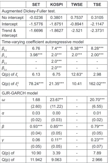
This paper provides the empirical study results of applying the time-varying coefficient autoregressive model and time- varying volatility model on four Asian stock market indices, Stock Exchange of Thailand (SET), Korea Composite Stock Price Index (KOSPI), Taiwan Stock Exchange (TWSE) and Tokyo Stock Exchange (TSE). The time-varying autoregressive model provides the evidences that Asian stock market indices have a non-linear dynamic relationship between current index and lagged periods indices. We also provide the evidence that the model can provide non- linear estimated mean which follow closely to the dynamic movement of the stock index. The GJR-GARCH which we employ in the conditional variance equation provide the evidence of the leverage effects in some markets.

This paper is organized as follows: Section II describes methodology while section III presents the Monte Carlo simulation results. Section IV presents the empirical results on Asian Stock markets. Finally, the summary is presented in the last section.

2. Research Methodology

For the traditional autoregressive model with lag order one or AR(1):

^y

^{= β}

^{+ β}

^y

^{+ ε}

(1) This AR(1) model has 2 parameters to be estimated β

and β

which can be easily estimated by linear least square method. The parameter β

shows how previous period of the

focused variable affect current period of the same variable.

However, these parameters are constant over-time. Under the stationary assumption, the parameter β

is required to have value in between -1 and 1 ( − < 1 β

< 1 ) . The ε

of the model is assumed to be a white noise series with zero mean and variance σ

ε (Tsay, 2002). Then, the mean µ and the variance σ

of the model in equation 1 are

( ) ( )

1

t t

E y E y µ β

β

=

= =

− (2)

( )

1

Var y

σ σ ^ε

= = β

− (3)

From equation 2 and 3, the parameter β

can’t be equal to +1 or -1, otherwise mean and variance of the AR(1) model will be explode to infinity. For the autoregressive with lag order greater than one, it is required that the characteristic roots of the parameter equation must be less than one in modulus (Chatfield, 2003; Hamilton, 1994; Tsay, 2002). For the time- varying autoregressive model with lag order one (TV-AR(1)):

y

= β

+ β

y

+ ε

(4) The parameters β

and β

now can be changing over time (Giraitis, Kapetanios & Yates, 2014). The ε

of the model is still assumed to be a white noise series with zero mean and variance σ

ε . Even though, the parameter β

can be changing over time, but the model still requires the value of parameter β

to be in between -1 and 1 (–1 < β

<1) (Dahlhaus, 1997). For the model with lag order greater than one, it is also required that the characteristic roots of the parameter equation must be less than one in modulus. Since the parameters of the new model now are time-variant, then mean and variance of the model can be changing over time (Giraitis, Kapetanios, & Yates, 2014).

1

t t

µ β

≈ β

− (5)

2 2

1,2 t

1

t

σ ε

σ ≈ β

− (6)

Bringmann et al. (2017) mentioned that, even though, the

model allows parameters to be changing over time, but it still

requires that the changing in parameters should be gradual

change and shouldn’t have a jump or sudden change in their

values. However, our Monte Carlo simulations show that,

even though, there is a sudden change or jump in parameter

value, the model still works very well. The time-varying

autoregressive model used the generalized additive model

(GAM) to estimate the time-varying parameters (Hastie

& Tibshirani, 1990; Sullivan, Shadish, & Steiner, 2015;

Wood, 2006). GAM applies the non-parametric smooth function that based on regression splines. For the simplified explanation, we follow Bringmann et al. (2017) to consider on time-varying coefficient autoregressive model with one a time-varying intercept and no autoregressive parameter.

y

= β

+ ε

(7)

By using regression splines method, the time-varying parameter can be estimate by

( ) ( ) ( ) ( )

0, 1 1 2 2 3 3

ˆ

ˆ R t ˆ R t ˆ R t ˆ

R t

β = α + α + α + +  α (8)

By choosing the type basis function R(K) and the number of basis function, k, then ˆ

β

can be estimated by using a simple linear regression.Each basis function can be calculated by the data we have, this method is actually a data driven approach. For a very simple example, we can choose a basis function as a polynomial with order 4, then R t =

( ) 1 ,

2

( )

R t = t , R t

( ) = t

, R t

( ) = t

, R t

( ) = t

(Wood, 2006).

The parameter ˆ

β

can be any shape from linear to any non-linear shapes. In practice, we have many choices on the type of basis function such as a cubic regression splines and thin-plate regression splines. In this paper, we use the package “mgcv” on R program to estimate the time-varying coefficient autoregressive model (Wood, 2006). We use a thin-plate regression splines which is the default setting on package because there are no need to choose the knot locations and it performs very well when we have many independent variables which, in our case, means it’s good for autoregressive with order greater than 1 (Wood, 2003).

The optimal value of estimated time-varying parameter ˆ

β

can be found when we perform the minimization of this penalized least squares loss function.

2 '' 2

0, 0,

1

+∞

= −∞

 

 −  +

   

∑

^y

^β

^λ ∫ ^β

^{dt (9)}

The first term equation 9 is a simple linear least square minimization. The second term is the roughness penalty or wiggliness. The smoothing parameter λ controls how the shape of time-varying parameter will look like. If λ is small, the wiggliness penalty will be small, then we will have a non- linear and wiggle shape of the parameter. On the other hand, if If λ is large, the shape of the parameter will be a straight line.

( )

( )

2 1 0,

2

ˆ

T

t t

T

y GCV tr I A

=

− β

=   −  

∑ ₍₁₀₎

The optimal value of λ can be achieved by choosing λ that give the lowest value of the generalized cross validation score (Wahba, 1980; Wood, 2006). After we perform the time-varying coefficient autoregressive model, we apply the Ljung-Box test on the estimated residuals and estimated squared residuals. If the model is adequate, there won’t have an auto correlation in the estimated residuals. If there is no heteroskedasticity problem, there won’t have an auto correlation in the estimated squared residuals (Tsay, 2002).

In the case that there is a heteroskedasticity problem, we will perform the time-varying volatility model. Glosten, Jagannathan and Runkle (1993)’s GJR-GARCH model will be used for the variance equation.

0, 1, 1

t t t t t

y = β + β y

+ ε (11)

( )

1/2

; ~ . . . 0,1

t

h z z

i i d

ε = (12)

2 2

1 1 1 1

t t t t t

h = + ω αε

+ γ I

ε

+ β h

(13) where I

= 0 , if ε

> 0 and I

= 1 , if ε

< 0 . Equation (11) is the conditional mean equation which follows the time-varying coefficient autoregressive model with lag order one. The mean equation can be easily extended to higher lag order. Equation (13) is the conditional variance equation which allow the variance, h

, to be changing over time under heteroskedasticity condition. We decide the use GJR-GARCH model for the variance equation because it extends Engle (1982)’s ARCH model and Bollerslev (1986)’s GARCH model to capture the different effect between positive and negative shocks on volatility. For the GJR-GARCH estimation, we use “rugarch” package on “R”

program which we decide to choose the generalized error distribution (GED) for the distribution option. GED offers some desirable benefits which can work with the data that has excess skewness and kurtosis.

3. The Monte Carlo Simulation Study

In this section, we provide the simulation study on the time-varying coefficient autoregressive model in order to show that the model can capture the dynamic movement of each parameter very well. The number of data in the simulation is 1,000 which follows the nature of financial data that has abundance of data available. The simulation will repeat 100 times and then calculates for 2.5%, 50%, 97.5% quantiles of each parameter and mean of the model.

We extend the simulation studied of (Bringmann et al., 2017)

to cover the model with lag order one, two and three. The

parameters of the model will follow fours cases: invariant

case, linear increasing case, sine function case and random

walk case.

For the invariant case, we set the parameters to be a fixed value. For the linear increasing case, we set the parameters to be increasing over-time in a linear form. For the sine function case, we set the parameters to be changing over-time in a non- linear form as a sine function; _{MAX sine .} ^{2. . t}

T π

   

 

   

  ,which

MAX is the maximum value of the parameter. The random walk case, we set the parameters to be changing over-time in a non- linear form with a sudden change or jump which follows the random walk process as β

= β

+ a

which α

has a normal distribution with zero mean and one standard deviation.

Time-varying coefficient autoregressive model with lag order one will follow equation 4. For the invariant case, the value of β

will be fixed at 3 while the value of β

will be equal to 0.7. For the linear increasing case, the value of β

will be linearly increasing from 0.5 to 3 while the value of β

will be linearly increasing from 0.3 to 0.7. For the sine function case, the value of β

and β

will follow sine function as MAX sine . 2. . t

T

 π 

 

  which MAX equal to 3 for β

and 0.7 for β

. For the random walk case, the value of β

and β

will follow random walk process with the maximum value equal to 3 and 0.7 respectively.

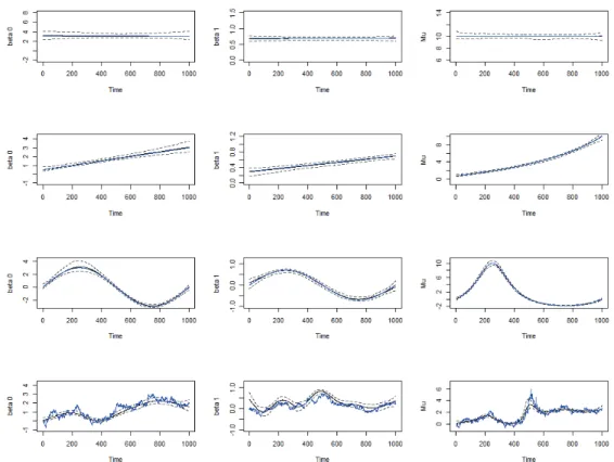
For Figure 1, the blue line is the real value while the black line is the 50% quantile from 100 times simulation and the dot lines are the 2.5% and 97.5% quantile from 100 times simulation. The first row of figure 1 shows the simulation results for the invariant case. Since β

and β

have a fixed value over time, then the mean of the model, µ, also has a fixed value over time. The second row shows the case that the parameter β

and β

are linearly increasing over time and the mean of the model, µ, is non-linear increasing over time with a positive time trend.

The third row shows that the model can reveal the sine shape of the parameters and the mean of the model very well. Even though, Bringmann et al. (2017) mentioned that the model is good if there is no jump or sudden change in the parameter, however, the last row shows that, for the case of random walk process in parameters, the model can capture the sudden change or jump in parameters and mean of the model very well.

Note: First row shows the parameters in theinvariant case. Second row shows the parameters in the linear increasing case. Third row shows the parameters in the sine function case. The fourth row shows the parameters in the random walk case. The first column shows the simulation results of β

while the second shows the results of β

. The third column shows the simulation results of the mean of the model, µ. Blue line is the real value while the black line is the 50% quantile from 100 times simulation and the dot lines are the 2.5% and 97.5%

quantile from 100 times simulation.

Figure 1: Simulation results of Time-varying coefficient autoregressive model with lag order one.

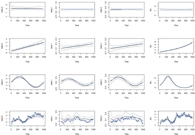
Time-varying autoregressive model with lag order two is shown in the following equation.

0, 1, 1 2, 2

t t t t t t t

y = β + β y

+ β y

+ ε (14)

For this model, we have 3 time-varying parameters to be estimated β

, β

and β

For the invariant case, the value of β

, β

and β

will be fixed at 3, 0.3 and 0.3 respectively.

For the linear increasing case, the value of β

will be linearly increasing from 0.5 to 3 while the value of β

and β

will be linearly increasing from 0.1 to 0.3. For the sine function case, the value of β

, β

and β

will follow sine function as MAX sine . 2. . t

T

 π 

 

  which MAX equal to 3, 0.3 and 0.3 respectively. For the random walk case, the value of β

, β

and β

will follow random walk process with the maximum value equal to 3, 0.3 and 0.3 respectively. Time-varying autoregressive model with lag order three.

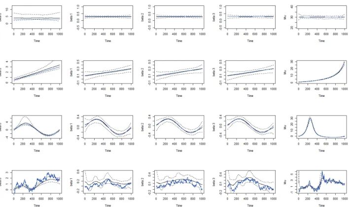
0, 1, 1 2, 2 3, 3

t t t t t t t t t

y = β + β y

+ β y

+ β y

+ ε (15) For this model, we have 4 time-varying parameters to be estimated β

, β

, β

and β

. For the invariant case, the value of β

, β

, β

and β

will be fixed at 3, 0.3, 0.3 and 0.3 respectively. For the linear increasing case, the value of β

will be linearly increasing from 0.5 to 3 while the value β

, β

and β

will be linearly increasing from 0.1 to 0.3. For the sine function case, the value of β

, β

, β

and β

will follow sine function as MAX sine . 2. . t

T

 π 

 

  which MAX equal to 3, 0.3, 0.3 and 0.3 respectively. For the random walk case, the value of β

, β

, β

and β

will follow random walk process with the maximum value equal to 3, 0.3, 0.3 and 0.3 respectively.

Figure 2 and 3 show the simulation results from the time- varying model with lag order two and three. The first row shows the invariant case while the second row shows the linear increasing case. The third row shows the sine function

Note: First row shows the parameters in the invariant case. Second row shows the parameters in the linear increasing case. Third row shows the parameters in the sine function case. The fourth row shows the parameters in the random walk case. The first column shows the simulation results of β

while the second shows the results of β

. The third column shows the simulation results of β

while the fourth shows the results of the mean of the model, µ. Blue line is the real value while the black line is the 50% quantile from 100 times simulation and the dot lines are the 2.5% and 97.5% quantile from 100 times simulation.

Figure 2: Simulation results of Time-varying coefficient autoregressive model with lag order two.

Note: First row shows the parameters in the invariant case. Second row shows the parameters in the linear increasing case. Third row shows the parameters in the sine function case. The fourth row shows the parameters in the random walk case. The first column shows the simulation results of β

while the second shows the results of β

. The third column shows the simulation results of β

while the fourth shows the results of β

. The fifth column shows the simulation results of the mean of the model, µ. Blue line is the real value while the black line is the 50% quantile from 100 times simulation and the dot lines are the 2.5% and 97.5% quantile from 100 times simulation.

Figure 3: Simulation of Time-varying coefficient autoregressive model with lag order three.

case while the last row shows the random walk case. As we can see, the model can reveal both linear and non-linear time-changing of the parameters and the mean of the model very well. For the random walk case, our simulation results provide the evidences that the time-varying coefficient autoregressive model work very well, even though, there is a sudden change or jump in parameters and model’s mean.

In addition, the model works very good on both stationary mean and non-stationary mean.

4. Empirical Study

In this section, we apply the time-varying coefficient autoregressive model to the stock market index in four Asian countries: Stock Exchange of Thailand Index (SET), Korea Composite Stock Price Index (KOSPI), Taiwan Stock Exchange Index (TWSE) and Tokyo Stock Exchange Index (TSE). For all 4 market, we use a daily time-series data from January 1, 2015 to February 12, 2020 which is acquired from Thromson Reuters. So, in total, we have 1,335 number of data on each market.

To check the stationary condition of the data on all 4 stock markets, we perform the Augmented Dickey-Fuller test (ADF test). According to the results in Table 1, we fail to reject the null-hypothesis of non-stationarity, so, we can conclude that the stock market indices in Thailand, South Korea, Taiwan and Tokyo, Japan are non-stationary. Since the time-varying coefficient autoregressive model can be applied to both stationary and non-stationary data, then, our model is appropriate for these stock market indices.

In order to get some information about the lag order

that we should use in the model, we perform the partial

autocorrelation function (PACF) (Tsay, 2002). For the

stock market in Thailand, Taiwan and Tokyo, we found the

significant PACF at lag order 1. For the stock market in South

Korea, we found the significant PACF at lag order 1, 3 and

4. Then, we perform time-varying coefficient autoregressive

model with many lags and check the significant level and

compare the value of AIC and BIC. Finally, we found that

the model with lag order one is appropriated for Thailand,

Taiwan and Tokyo while the model with lag three is

appropriated for the South Korea.

Table 1: Time-varying coefficient autoregressive model and time-varying volatility model results

SET KOSPI TWSE TSE

Augmented Dickey-Fuller test.

No intercept -0.0236 0.3801 0.7537 0.3105 Intercept -1.5776 -1.8751 -0.8941 -2.1147 Trend &

intercept -1.6696 -1.8627 -2.521 -2.3731 Time-varying coefficient autoregressive model

β

6.76 7.4*** 6.38*** 8.28***

β

3.98*** 2.0*** 2.0*** 2.00***

β

- 2.0*** - -

β

- 2.0*** - -

Q(p) of ε̂

6.13 6.75 12.63* 2.98

Q(p) of ε̂

78.24*** 21.35*** 10.41 162.02***

GJR-GARCH model

ω 1.68 23.67** - 20.70***

(2.60) (11.22) - (6.55)

α 0.03 0.00 - 0.01

(0.02) (0.03) - (0.02)

β 0.93*** 0.85*** - 0.79***

(0.04) (0.05) - (0.05)

γ 0.06 0.11** - 0.23***

(0.05) (0.05) - (0.07)

Q(p) of 10.90 3.39 - 7.89

Q(p) of 11.942 9.063 - 2.966

Note: The Augmented Dickey-Fuller test statistics are reported in the first three row with the null hypothesis of non-stationarity. For the time-varying coefficient autoregressive model in conditional mean equation, the values in the row of β

, β

, β

and β

are EDF which refer to the number of basis functions that are used to estimate the time-varying coefficient in the model. Q(p) and Q

(p) are Ljung-box test for the p

order serial correlation with the null hypothesis of no autocorrelation. For the GJR-GARCH model in conditional variance equation, the robust standard errors are reported in parenthesis. Asterisks indicate statistical significance for the rejection of null hypothesis at 10% (*), 5% (**) or 1% (***) level.

SET stands for Stock Exchange of Thailand Index while KOSPI stands for Korea Composite Stock Price Index. TWSE stands for Taiwan Stock Exchange Index while TSE stands for Tokyo Stock Exchange Index.

The results of the time-varying coefficient autoregressive model and time-varying volatility model are reported in table 1 and figure 4. For table 1, the values in the row of β

, β

, β

and β

are effective degrees of freedom (EDF). Since we use the regression splines method to estimate the time-

varying parameter which comes from the summation of basis functions that is shown in equation 8, the effective degrees of freedom (EDF) refers to the number of basis functions that use to estimate the parameter. The default number of basis function in “mgcv” package is 10, however, the number of basis function that need in model is referred to EDF. The high number of EDF means the model uses many basis functions to estimate the parameter, then we will have the non-linear and wiggly shape of the parameter. On the other hand, if the EDF is close to 1, we will have the linear shape of the parameter (Shadish, Zuur, & Sullivan, 2014). In additional, asterisks in table 1 refer to the rejection of null-hypothesis which means that the smooth time-varying parameter is significantly different from zero (Wood, 2013). According to table 1, all of the estimated time-varying coefficients in four Asian stock market indices are significantly different from zero except the intercept of Thailand case.

For the model checking, if the time-varying coefficient autoregressive model in conditional mean equation is adequate, then the estimated residuals () of the model should behave like a white noise with no auto-correlation (Tsay, 2002). The Ljung-Box tests on the estimated residuals ( ε ˆ

) are shown in the row of “Q(p) of ε ˆ

”. For the case of SET, KOSPI and TSE, there are no autocorrelation in the estimated residuals which means the time-varying coefficient autoregressive model in conditional mean equation is adequate while, for the case of TWSE, there still has an autocorrelation with 10% significant level.

To check the heteroskedasticity problem, we perform the Ljung-Box tests on the squared estimated residuals ( ε ˆ

) and report the results in the row of “Q(p) of ε ˆ

”. The results suggest that there is an autocorrelation in squared estimated residuals in the case of SET, KOSPI and TSE which means we need to construct the time-varying volatility model to capture the heteroskedasticity condition. For the lower part of table 1, we provide the results of GJR-GARCH model for the case of SET, KOSPI and TSE. However, we didn’t do the GJR-GARCH model on TWSE since there is no heteroskedasticity problem for Taiwan. The significant results of estimated parameter β suggest that the volatility of the stock market today has a highly correlated with the volatility yesterday while the significant results of estimated parameter γ suggest that the negative shock has more impact on market’s volatility than positive shock in KOSPI and TSE.

If the conditional variance equation is adequate, the estimated standardized residual ( z ˆ

) and estimated squared standardized residual ( z ˆ

) shouldn’t have an autocorrelation problem (Tsay, 2002). We perform the Lung-Box test on estimated standardized residual and estimated squared standardized residual. The results in the row of “Q(p) of z ^ˆ

” and “Q(p) of z ˆ

” suggest that there is no autocorrelation

in standardized residual and squared standardized residual which means that our GJR-GARCH model in conditional variance equation is adequate.

The results of time-varying parameters on SET, KOSPI, TWSE and TSE are shown in Figure 4. The solid black line is the estimated time-varying parameter of the model while space between the dot lines is 95% confidence interval. We use bootstrap resampling residuals approach to estimate the confidence interval (DiCiccio & Efron, 1996). Firstly, we estimate the model to get the fitted values y ˆ

and the residuals ε = − ˆ

y y

ˆ

. Secondly, we randomly resample the residuals, ε ˆ

and create the new variable y

= y ^ˆ

+ ε ^ˆ

. Thirdly, we estimate the model on the new variable y

to get the new estimated parameters. Finally, we repeat step 1 to 3 for 1,000 times and calculate the 2.5% and 97.5% quantile of 1,000 times bootstrapping parameters to get the confidence interval.

Figure 4 shows the estimated time-varying coefficients of Stock Exchange index of Thailand, Taiwan, Tokyo and South Korea. For Thailand, Taiwan and Tokyo, the time-varying coefficient autoregressive with lag order one is preferred. For Thailand, the stock index yesterday had a strong effect on the

index today and this effect was increasing from 2015 to 2018 and then started to decline until 2020. For Taiwan, the effect of 1 previous period index on current index had a small decreasing over time. For Tokyo, the effect of 1 previous period index on current index had a time-invariant at 0.96.

For South Korea stock market, the time-varying coefficient autoregressive with lag order three is preferred. The effect of 1 previous period index on current index was decreasing over time while the effect of 2 period lagged index on current index was increasing. The effect of 3 period lagged index on current index was deceasing over time. For South Korea, the stock index yesterday had a strong effect on the index today while the index two and three day ago had only a small effect on the index today.

By using equation 5, we can calculate the time-varying mean of the model. We show the estimated mean of the model in the black line along with the stock index in the blue line in Figure 5. As we can see, the time-varying coefficient autoregressive can reveal the dynamic movement of estimated mean very well in all 4 Asian stock markets. The estimated mean can reveal the downturn and the upturn of the market very well which the traditional autoregressive cannot do.

Note: The solid black line is the estimated time-varying coefficient of the model while space between the dot lines is 95% confidence interval.

Figure 4: Time-varying coefficients of Stock Exchange of Thailand Index (SET), Taiwan Stock Exchange Index (TWSE),

Tokyo Stock Exchange Index (TSE) and Korea Composite Stock Price Index (KOSPI).

5. Conclusions

In this paper, we show a Monte Carlo simulation study and an empirical study of the time-varying coefficient autoregressive model. Our simulation shows that the estimated parameters of the time-varying autoregressive model can reveal the true shape of parameters and mean of the model very well, even though, there are some sudden change or jump. The model can be applied to both stationary time- series data and non-stationary data that have a time-trend. Our simulation shows the results from the time-varying coefficient autoregressive model with lag order one, two and three.

We also provide the results of applying the time- varying autoregressive model on four Asian stock markets.

We found that Stock Exchange of Thailand Index, Taiwan Stock Exchange Index and Tokyo Stock Exchange Index can be explained very well by the time-varying coefficient autoregressive with lag order one while South Korea Stock Exchange Index can be explained by the model with lag order three. For the case of South Korea and Tokyo, we found that the negative shocks have more impact on market’s volatility than positive shock. We found that the time-varying mean of the model follows the non-linear pattern of stock market index very well in all 4 markets.

References

Bollerslev, T. (1986). Generalized autoregressive conditional heteroskedasticity. Journal of Econometrics, 31(3), 307–327.

Bringmann, L. F., Hamaker, E. L., Vigo, D. E., Aubert, A., Borsboom, D., & Tuerlinckx, F. (2017). Changing dynamics:

Time-varying autoregressive models using generalized additive modeling. Psychological Methods, 22(3), 409–425.

Chatfield, C. (2003). The analysis of time series: An introduction (5th ed.). Boca Raton, FL: Chapman and Hall/CRC.

Chow, S.-M., Zu, J., Shifren, K., & Zhang, G. (2011). Dynamic factor analysis models with time-varying parameters.

Multivariate Behavioral Research, 46(2), 303–339.

Dahlhaus, R. (1997). Fitting time series models to nonstationary processes. The Annals of Statistics, 25(1), 1–37.

DiCiccio, T. J., & Efron, B. (1996). Bootstrap confidence intervals (with Discussion). Statistical Science, 11, 189–228.

Engle, R. F. (1982). Autoregressive conditional heteroscedasticity with estimates of the variance of United Kingdom inflation.

Econometrica, 50(4), 987–1007.https://www.jstor.org/

stable/1912773

Giraitis, L., Kapetanios, G., & Yates, T. (2014). Inference on stochastic time-varying coefficient models. Journal of Econometrics, 179(1), 46–65.

Glosten, L. R., Jagannathan, R., & Runkle, D. E. (1993). On the relation between the expected value and the volatility of the nominal excess return on stocks. The Journal of Finance, 48(5), 1779–1801.

Goudarzi, H., & Ramanarayanan, C. S. (2010). Modeling and Estimation of Volatility in the Indian Stock Market.

International Journal of Business and Management, 5(2).

DOI:10.5539/ijbm.v5n2p85

Hamilton, J. D. (1994). Time series analysis. Princeton, NJ:

Princeton University Press.

Hastie, T. J., & Tibshirani, R. J. (1990). Generalized additive models. Boca Raton, FL: Chapman and Hall/CRC.

Ismail, M. T., & Isa, Z. (2008). Identifying regime shifts in Malaysian stock market returns. International Research Journal of Finance and Economics, 15, 1450-2887.

Lee, J. W., & Brahmasrene, T. (2018). An exploration of dynamical relationships between macroeconomic variables and stock prices in Korea. Journal of Asian Finance, Economics and Business, 5(3), 7-17. http://doi.org/10.13106/jafeb.2018.vol5.

no3.7

Note: Blue line is the stock market index while the black line is the estimated mean of the model and space between dot lines are 95%

confidence interval.

Figure 5:Time-varying mean of Stock Exchange of Thailand Index (SET), Taiwan Stock Exchange Index (TWSE), Tokyo

Stock Exchange Index (TSE) and Korea Composite Stock Price Index (KOSPI).

Lee, J. W., & Zhao, T. F. (2014). Dynamic relationship between stock prices and exchange rates: Evidence from Chinese stock markets. Journal of Asian Finance, Economics and Business, 1(1), 5-14. https://doi.org/10.13106/jafeb.2014.vol1.no1.5.

Parsva, P., & Lean, H. H. (2017). Multivariate causal relationship between stock prices and exchange rates in the middle east.

Journal of Asian Finance, Economics and Business, 4(1), 25-38. http://dx.doi.org/10.13106/jafeb.2017.vol4.no1.25 Shadish, W. R., Zuur, A. F., & Sullivan, K. J. (2014). Using

generalized additive (mixed) models to analyze single case designs. Journal of School Psychology, 52(2), 149–178.

Sullivan, K. J., Shadish, W. R., & Steiner, P. M. (2015). An introduction to modeling longitudinal data with generalized additive models: Applications to single-case designs.

Psychological Methods, 20(1), 26–42.

Tsay, R. S. (2002). Analysis of financial time series. Hoboken, NJ:

John Wiley & Sons, Inc.

Wahba, G. (1980). Spline bases, regularization, and generalized cross validation for solving approximation problems with large quantities of noisy data. In: E. Cheney (ed.), Approximation Theory III. London, UK: Academic Press.

Wasim, A., & Bandi, K. (2011). Identifying regime shifts in Indian stock market: A Markov switching approach. MPRA Paper ID 37174. Retrieved from https://mpra.ub.uni-muenchen.de/id/

eprint/37174.

Wood, S. N. (2003). Thin plate regression splines. Journal of the Royal Statistical Society, Series B, 65, 95-114.

Wood, S. N. (2006). Generalized additive models: An introduction with R. Boca Raton, FL: Chapman and Hall/CRC.

Wood, S. N. (2013). On p-values for smooth components of an

extended generalized additive model. Biometrika, 100(1),

221–228.