Broken Detection of the Traffic Sign by using the Location Histogram Matching

(1)

Liu Yang^†, Suk-Hwan Lee^††, Seong-Geun Kwon^†††, Kwang-Seok Moon^††††, Ki-Ryong Kwon^{†††††}

ABSTRACT

The paper presents an approach for recognizing the broken area of the traffic signs. The method is based on the Recognition System for Traffic Signs (RSTS). This paper describes an approach to using the location histogram matching for the broken traffic signs recognition, after the general process of the image detection and image categorization. The recognition proceeds by using the SIFT matching to adjust the acquired image to a standard position, then the histogram bin will be compared preprocessed image with reference image, and finally output the location and percents value of the broken area. And between the processing, some preprocessing like the blurring is added in the paper to improve the performance. And after the reorganization, the program can operate with the GPS for traffic signs maintenance. Experimental results verified that our scheme have a relatively high recognition rate and a good performance in general situation.

Key words: Road image recognition, Traffic sign, Histogram matching, SIFT features, Broken detection

※ Corresponding Author : Kwang-Seok Moon, Address : 599, Daeyeon-dong, Namgu, Busan, Korea (608-737), TEL: 051)629-6218, FAX : 051)629-6210, E-mail : ksmoon

@pknu.ac.kr

Receipt date : Sep. 2, 2011, Revision date : Dec. 19, 2011 Approval date : Dec. 25, 2011

†††††Master's degree, Dept. of IT Convergence and A- pplication Engineering, Pukyong National Universi- ty Korea (E-mail: [email protected])

†††††Associate Professor, Dept. of Information Security, Tongmyong University, Korea

(E-mail : [email protected])

†††††Assistant Professor, Dept. of Electronics Engineer- ing, Kyungil University, Korea

†††††Professor, Dept. of Electronics Engineering, Puk- yong National University Korea

†††††Professor, Dept. of IT Convergence and Application Engineering, Pukyong National University Korea

※ This work was supported by the “Human Resource Development Center for Economic Region Leading In- dustry” Project, supported by the Ministry of Education, Science & Technology (MEST) and the National Research Foundation of Korea (NRF) and also MEST and NRF through the Human Resource Training Project for Regional Innovation.

1. INTRODUCTION

Traffic signs are an important part of any

roadway. These signs are an inherent part of the traffic environment. They are designed to regulate the flow of vehicles. They give specific information to the road users, or warn against unexpected road circumstances. Perception and fast interpretation of the road signs is crucial for the driver’s safety.

These signs provide critical information to drivers on the roadway. Traffic signs are a safety pre- caution as well as an informational resource. But sometimes because of the weather or vandalism there are some signs which may be broken. Then the sign recognition for the driver can be tough.

It will jeopardize the driver’s estimations, even cause an accident. So keeping traffic signs well maintained and easily viewable is an important matter that benefits everyone who is the traffic participants. So that in time detect the broken traffic signs and maintain them is very necessary.

While we check the traffic sign by people, it’s need lots of workload and time. Then we hope to use an automatic approach to deal with the broken detection.

(2)

In the traffic sign recognition, various methods and techniques have been researched. Zhu et al.

presents the color-geometric model for traffic sign recognition [1]. Lee et al. recognize the traffic sign by dividing characters and symbols regions [2].

And some other way like [3] Most of them can be divided into two stages: Image detection and image categorization. After that we propose a next stage for detecting the broken area.

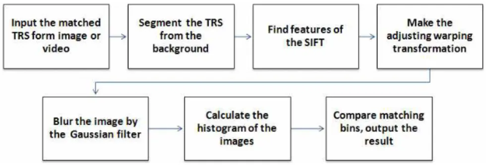
The paper describes an approach as the third stage. That initially segments the traffic signs from the background. Use the SIFT features to adjust the image which is acquired scaling or rotation to the standard camera axis orientation, and then blur the image for eliminating the noise parts.

Next calculates the histogram of the acquired and referenced image. Compare the two images to find the difference. Finally the program outputs the location and percentage of the broken area. And the advantage of this approach is that it can process the data in time when the carrier car is moving at regular speed. And it can modify the recognition accuracy according to the requirements. The part which needs to improve is the SIFT features do not have a satisfied matching success rate in some situations.

2. Related works

2.1 SIFT algorithm

There is an important part in the paper is SIFT algorithm. About the SIFT, Author David G. Lowe published a classic article is the distinctive image features from scale-invariant keypoints[4]. And the object recognition from local scale-invariant features[5]. The articles explain the SIFT algorithm in detail. SIFT keypoints of objects are first extracted from a set of reference images and stored in a database. An object is recognized in a new image by individually comparing each feature from the new image to this database and finding candidate matching features based on Euclidean dis-

tance of their feature vectors. The determination of consistent clusters is performed rapidly by using an efficient hash table implementation of the gen- eralized Hough transform. Each cluster of 3 or more features that agree on an object and its pose is then subject to further detailed model ver- ification and subsequently outliers are discarded.

Finally the probability that a particular set of features indicates the presence of an object is com- puted, given the accuracy of fit and number of probable false matches. Object matches that pass all these tests can be identified as correct with high confidence. The SIFT feature is invariant to the rotation and scale; it is robust to added noise, viewpoint change and the illumination change. It is possible to achieve image registration successfully when large scale change occurs. And another characteristic of the SIFT is that it have a good accuracy efficiency and speed. The algorithm has a reliable pose models and better error tolerance with fewer matches. Using the SIFT algorithm, It is convenient for us to find the unique feature pointers on the images.

2.2 Traffic sign recognition

In the Traffic Sign Recognition phase, we can see there are a lot of papers about this. Some of them separately use color features or shape features to make the pattern matching. And some match use an image to patch against an input image by “sliding” the path over the input image.

They can process the data in time, meanwhile have a good performance. We reference the general traffic sign recognition by feature matching proposed by Ren et al.[6], and the Automatic Detection and recognition of traffic signs using geometric structure analysis by Vavilin et al.[7]. In the first paper potential signs are compared with the tem- plate traffic signs as given in the database by using feature matching methods (SIFT or SURF feature)[8,9]. There are many contents is similar between the previous paper and this paper. In the re-

(3)

Fig. 1. The process of proposed scheme.

alization phase, this feature is going to make it easier. But there is a problem, when there is not only traffic sign in the image, especially the sign is similar. The program will confuse with that.

However the traffic signs recognition system has already been a very mature system. There are many approaches and algorithms to realize the recognition phase. The previously mentioned article is part of the paper which is we referenced[10-15].

On this basis, we propose an approach to recognize the broken area on the traffic signs.

In the traffic sign maintenance, a necessary part is the broken traffic sign detection. Usually this part is passively depending on the traffic participants or the period maintenance. That can’t only deal with the broken in time and accurately, and that will take lots of time and labor. So we extend the traffic sign recognition system to the broken detection phase. We hope that it can bring more environment and economy benefit.

3. Proposed scheme

People estimate if a traffic sign is broken is according to their memory. Because they have already known what the perfect traffic sign should be. Then they compared the sign which they found with the one in memory. So a direct easy way for detecting broken sign is compare the traffic sign with a reference. The acquired image may be acquired by any camera axis orientation. So we, according to the SIFT features transform the image to the reference image position. For locating the

broken area we split image by N bins along the x and y axis of the image. Subsequently we can compare the bins which are separate from the acquired image and the reference. Then we can know if the same number bin has a different value. Then this number row or column must have the broken area. That is the brief idea about the paper.

3.1 SIFT features

In order to obtain the broken information, the most direct way is to adjust the traffic road signs to the standard camera axis orientation, and then compare with reference image. So at the initial stage, the method of image warping transformation requires some unique character of the points to make the mapping. Then the SIFT feature is brought in method. The SIFT feature is invariant to the rotation and scale, as well as it is robust to added noise, viewpoint change and the illumination change. It is possible to achieve image registration successfully when large scale change occurs.

The SIFT consist of four major stages:

(1) scale-space peak selection (2) keypoint localization (3) orientation assignment (4) keypoint descriptor

In the first stage, potential keypoints are identified by scanning the image over location and scale.

In the second stage, candidate keypoints are lo- calized to sub-pixel accuracy and eliminated if found to be unstable. The third identifies the domi- nated orientations for each keypoint based on its

(4)

local image patch. The assigned orientations, scale and location for each keypoint enables SIFT to construct a canonical view for the keypoint that is invariant to similarity transforms. The final stage builds a local image descriptor for each keypoint, based upon the image gradients in its local neighborhood. According to the keypoint descriptor, we can match two images. But in general, there is still some limitation about images which we acquired from the natural.

For example, image matching succeeds between day images and between night images. However, under day-and-night illumination change, the method may fail. There is a situation is one image general image, but the other is in close-up shows strong relief effect. And due to the viewpoint change, the SIFT find less matches (Fig. 2).

Fig. 2. Matching performance according to viewpoint angle.

3.2 Warping transformation

When people don’t look straight at the plane of the traffic sign, the view will like the Fig. 3 (b).

It’s a random position. But because of the method requirement, we use a geometric manipulation to transform the traffic sign to the special position.

It maps pixels from one location to a different location, often performing subpixel interpolation along the way. According to the SIFT feature points, we can compute the actual transforms that relate the different views. In this paper perspective trans- formations are used to model the views. After we

have the parameters of the matched feature points, we use the function cvWarpPerspective from the OpenCV to turn the acquired image to the standard camera axis orientation.

(a) (b)

Fig. 3. Correspondence of SIFT in different images (a) Warping transformed image and (b) captured signature image.

3.3 Blurring

Before we calculate histogram of image we need some preprocessing. For example the smoothing, also called blurring, it is a simple image processing operation. There are many reasons for smoothing, but it is usually done to reduce noise or man-made errors. In our case, because the manufacture or some previous processing, most of times, we can’t get the exactly perfect matching sample. So we use the blurring to deal with the mismatching edge of the images and noise. We select the Gaussian filter.

It is probably is not the fast but the most useful.

Gaussian filter has nice properties, such as having no sharp edges, and thus does not introduce ringing into the filtered image. A Gaussian blur effect is typically generated by convolving an image with a kernel of Gaussian values. How should we define the kernel value? We need according to the experi- ence to separate which kind of situation is noise and which is broken to decide how strong of the kernel of Gaussian values. In this paper, we built the kernel. The kernel size was defined by 7×7.

And the kernel value was defined by 2. In the figure 4, we can see the different image (a) without blurring have the mismatching edge which has been signed by circle. But the blurring image eliminates that part difference.

(5)

3.4 Calculate 2D histogram

Histogram is a graphical representation, show- ing a visual impression of the distribution of data.

We know that the original histogram is used to reflect pixels gray level distribution while dealing with the image. The horizontal axis is the gray level, and the vertical axis is the number of pixels.

But in this paper we want the histogram to reflect the information about the location of the pixels. So the original image histogram was improved with the location horizontal axis histogram.

(a) (b)

Fig. 4. Two cases (a) without blurring and (b) with blurring.

Fig. 5. Example of collection of the TRS in different situation.

3.4.1 Divide color range

Before we built the histogram, we needed to divide the color range, to tell the program what kind of color pixels could be counted. The color range division is in the RGB model. Due to varying light and weather conditions, the division of traffic signs using color information; especially in outdoor images is a significantly challenging task. So the paper attempts to collect every condition with the ul- timate aim to make sure the color range is complete. The conditions contain day, bad light, high light, fading, fog, and the reflection from cars.

We divide the color range according to some ulti-

mate sample. Then we get the five kinds of the general traffic sign color in RGB model.

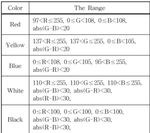
After then, we divide the color range as the table 1. In the RGB model we limit the red, green and blue tricolor’s value according to the previous situation. And meanwhile limit the absolute difference value. In this way we can express the color range. In table 1, the value is from the various samples’ the RGB value and select the extremity one in them. Here we can get the white and black’s range is obvious near. Such low contract always appears especially in some fog weather.

Color The Range

Red 97<R≤255, 0≤G<108, 0≤B<108, abs(G-B)<20

Yellow 137<R≤255, 137<G≤255, 0≤B<105, abs(G-R)<20

Blue 0≤R<108, 0≤G<105, 95<B≤255, abs(G-R)<20

White 110<R≤255, 110<G≤255, 110<B≤255, abs(G-B)<30, abs(G-R)<30,

abs(R-B)<30,

Black 0≤R<100, 0≤G<100, 0≤B<100, abs(G-B)<30, abs(G-R)<30, abs(R-B)<30,

Table 1. The available range of each color

3.4.2 2D Histogram

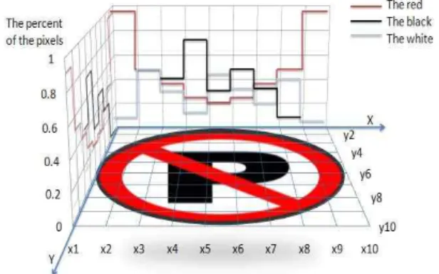
After that we calculate the histogram. The approach builds the histogram respectively along the horizontal and vertical lines of the image, and then we can get a model like figure 6. In view of the image size of this paper, as you can see the image was divides by 30. We chose this number because it can accurately respond the differences; meanwhile the program can have a good processing time. We established that the x would denote the horizontal axis, and the y would denote the vertical axis of the image. If the reference or the warp transformed image size is NH×NV. Then the size of every block in the image will be NH/30 × NV/30.

(6)

Every block can be labeled by ^{}.

From the image we can see that the ban park sign has been divided into the blocks with the square of bin numbers. Therefore we calculate the histogram along the x and y axis. We can get the percentage of the pixels of each color. The estimate if the cell is broken is according to the row and the column which crosses the block. In the next stage we are going to compare with the reference by the same number bin value. We suppose that if the difference value of the same number bin is out of the range then it is broken. X histogram for row array, Y histogram for column array. Assume that 2D histogram X·Y is denoted by ^{} with.

∈ Define 2D histogram by equation:

X- color histogram

  ____{}_

_  

_^∆^{}

_{   ∆}^∆ ^{}

(1)

Y- color histogram

  ____{}_

_  

_^∆^{}

_{   ∆}^∆ ^{}

(2)

In Fig. 6, the ban park sign has been divided into the blocks with the square of bin numbers. Because the ban park sign only has three kinds color. We only calculate three kinds of histogram. If there is any kind of 5 kinds color, they will be calculated.

We only count the pixels on the sign. It not contain the pixel which is out of the sign range but in the X·Y matrix range. That’s why the a bit of red pixels have a high percentage at both ends of the histogram.

3.5 Compare matching bins

After we use this model histogram to calculate

Fig. 6. The 2D location histogram model.

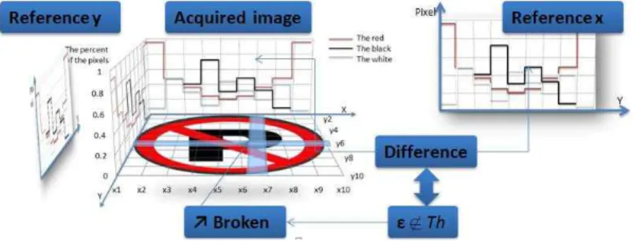
the acquired image and the reference images, the program respectively compares the horizontal and vertical axis of the acquired image with the reference. In this way we can get the difference of the bins of the rows and columns. Then we can locate the broken cell by the broken rows and columns. Those cross cell will be the broken one.

The ^{} is histogram of reference image, the

′′ is histogram of captured image, then

_  ′_  _ _  ′_  _ (3) with∈ ∈

_ 

 if and_ 

 

(4)

_ is the absolute difference value of the bins in the same orientation. We calculate in this way with 5 kinds of color, then we calculate the broken maps for 5 Colors:^___{}_. Finally the broken map is according to ^{  }___{}_ (|| : in- clusive OR). In the equation, initially we calculate the individual color, then combine the result by the OR logical operation. ^ is the output matrix, in the matrix we use 1 to denote the broken cell, and use 0 to denote the unbroken.Th is the threshold which we defined. This threshold is an error re- dundancy value which we can accept. In the program part we defined it is the 5 percent of the number of pixel in the cell.

(7)

Fig. 8. The whole broken area detection step

Fig. 7. The difference compare step.

4. Result and Analysis

Fig. 8 shows an example of the broken recognition. In this paper 60 images were used for testing. And the size is from 160×160 to 560×560 pixels. The samples contain the warning sign, pro- hibitory sign and mandatory sign; meanwhile the samples contain the red, yellow, blue, white and black five kinds of regular color. And we consider about the illumination and white balance, so the samples are captured in different weather. The condition contains day, bad light, high light, fading, the fog, and the reflections from cars. In the test samples we select some signs and captured them from different camera axis orientations. In the paper we test the `performance criterion about the response time and matching rate with different

situations.

4.1 Processing time

First of all is the processing time, we test the different warning sign, mandatory sign and pro- hibitory sign with different size. And the result is given in the Fig. 9.

The time is without the traffic sign recognition phase, only the broken recognition phase. If we use bigger or more complicated images, the program will take more time.

Fig. 9. The processing time.

4.2 Matching rate, (broken area)

Base on the previous contents we can write the broken area:

 



  ^

_{  }^^{}



^×∆^ ⁽⁵⁾

Then the percentage of broken area PBA:

   ×

  (6)

We measure if the match is right or wrong ac-

(8)

0 10 20 30 40 50 60 70 80 90 100

The day Bad light High light The faded The fog Reflection from car

Matching rate (%)

The illumination situation Fig. 10. The matching rate in different situation.

0 20 40 60 80 100

0 10 20 30 40 50 60 70 80 90

Matching rate (%)

Viewpoint angle (degrees) Fig. 11. The viewpoint angle influence.

cording to the above equation. If the mismatching is less than the 10 percent of the image area, we think the match is successful.

About the matching rate we separately test in different environment and camera axis orientations.

The illumination will influence two parts of the system. One of them is the day-and-night kind of illumination difference that may make the SIFT feature matching fail. And the other is the different illumination that was influence on the number of bins in the histogram.

In Fig. 10, we can see two bad conditions: bad light and fog. In general, matching succeeds between day images and between night images, but when the acquired image is from night and match it with the day reference, the methods will fail. In the fog day the color contrast will be small. That makes some color out of the color range which we defined, especially the white and black.

From the Fig. 10 we know the system have a good performance in most cases. But we also see actually the system can’t work under the bad light and fog.

The camera axis orientation is a big influence element of the SIFT matching phase. As we previously mentioned the matching rate will be lower with view point angle rise. But in Fig. 11 this element reflects to the whole system, it has a worse performance. Because it’s not only we can’t get the

matched couple, it also has some “good” false matches. In the warping transformation phase we need to select four pairs matched points to make the transformation. If there are one “good” false matching point that is selected the transformed traffic sign will still have some perspective warping. If there is more than one of this kind of false matching points the transformation will be totally messed up.

We first use the histogram calculation of the acquired image and the reference. And then compare them. In this paper we divide the image by thirty bins. The bin number in one side depends on the accuracy which we required. The other side is that we need consider about a problem. If the grid is too wide, then there is too much averaging and we lose the structure of the distribution. If the grid is too narrow, then there is not enough averaging to represent the distribution accurately and we get small, “spiky” cells.

Because there are some noise like ring is im- ported into the image. Sometimes in the result we will see that the matrix will show another small

“broken” area beside the real broken one. When we calculate the pixel number, these area pixels may overflow its original color range. Then this kind of difference may be recorded in the matrix.

4.3 compare with other method

We compare our method with other broken detection. For example in the , D. M. Tsai[16] pro-

(9)

poses a way to detect the defection in low-contrast surface images of the Liquid Crystal Display (LCD). A constrained ICA model has been proposed for the design of the convolution filter. The proposed ICA-based filtering scheme can effec- tively detect various defects in low-contrast textured surface images. But it is too sensitive for the traffic sign which is from the outdoor. Meanwhile, it need more time than our method. And we also compare with, Oprea[17] propose an application for detection of broken Aspirin tablets. Somewhere of the paper is similar to our method. But we have better performance in solving noise and random position.

5. CONCLUSIONS

The paper presents an approach to detect the broken information of the traffic signs. Initially we get the matched traffic sign image. And next find the SIFT features from both the acquired image and the reference; Next we transform the acquired traffic sign image to the standard camera axis orientation, we blur both images to eliminate the noises. And then compare the acquired image with the reference by using the position histogram.

Finally we output the location and the percentage of broken parts

The approach in this paper only presents a brief way to detect the broken area. We can do some preprocessing to make this system more accurate.

And another part that is worth to improve is the SIFT features matching. We can combine the Harris pointer or some geometric limited to improve the accuracy rate of the matching. Another way is that the approach in the paper can change the SIFT features to the Affine-SIFT (ASIFT).

While SIFT is fully invariant with respect to only four parameters namely zoom, rotation and trans- lation, the ASIFT treats the two left over parameters: the angles defining the camera axis orientation. Against any prognosis, simulating all

views depending on these two parameters is feasible. About the color segmentation in the paper we limited the color range in the RGB model.

Subsequently we can attempt on another color model and import the white balance element to make the program work more accurately.

REFERENCES

[ 1 ] S.D. zhu, L.L. Liu, and X.F. Lu, “Color- Geometric Model for Traffic Sign Recogni- tion,”IMACS Multiconference on CESA, pp.

2028-2032, 2006.

[ 2 ] J.H. Lee and K.H. Jo, “Traffic Sign Recognition by Division of Characters and Symbols Regions,”Proc. KORUS 2003, Vol.2, pp. 324-328, 2003.

[3] J.D. Jeon, M.J. Lee, J.H. Kim, S.K. Kim, B.D.

Kang, “An Object Dection System using Eigen-background and Clustering,”Journal of Korea Multimedia Society, Vol.13, No.1, pp.47-57, Jan. 2010. (멀티학회 논문지 추가) [ 4 ] D.G. Lowe, “Distinctive Image Features from

Scale-Invariant Keypoints,” ACM Int’I J . Computer Vision, Vol.60, No.2, pp. 91-110, 2004.

[ 5 ] D.G. Lowe, “Object Recognition from Local Scale-Invariant Features,” Proc. Int’l Conf.

Computer Vision (ICCV), pp. 1150-1157, 1999.

[ 6 ] F.X. Ren and J.h. Huang, “General Traffic Sign Recognition by Feature Matching,”24th International Conference Image and Vision Computing, pp. 409-414, 2009.

[ 7 ] V. Andrey and K.H. Jo, “Automatic Detection and Recognition of Traffic Signs using Geometric Structure Analysis,”SICE-ICASE International Joint Conference, pp. 1450-1456, 2006.

[ 8 ] M. Teke and A. Temizel, “Multispectral Satellite Image Registration using Scale- Restricted SURF,”Pattern Recognition (ICPR), pp. 2310-2313, 2010.

(10)

[ 9 ] S.L. Huang and C.Cai, “An Efficient Wood Image Retrieval using SURF Descriptor,”

Test and Measurement ICTM’09, pp. 55-58, 2009.

[ 10 ] S.D. Zhu and L.L. Liu, “Traffic Sign Recognition based on Color Standardization,”

P roc. of the 2006 IEEE International Conference on Information Acquisition, pp.

951-955, 2006.

[11] B.V. Funt and G.D. Finlayson. “Color Constant Color Indexing,” IEEE Transactions on Pattern Analysis and Machine Intelli- gence, Vol.17, No.5, pp. 522-529, 1995.

[12] A.E. Johnson and M. Hebert, “Using Spin Images for Efficient Object Recognition in Cluttered 3D Scenes,”IEEE Transactions on P attern Analysis and Machine Intelligence, Vol.21, No.5, pp. 433-449, 1999.

[13] A. Diplaros and T. Gevers, “Combining Color and Shape Information for Illumination- Viewpoint Invariant object Recognition,”

IEEE Transactions on Image P rocessing, Vol.15, No.1, pp. 1-11, 2006.

[14] S. Abbasi and F. Mokhtarian, “Affine-Similar Shape Retrieval: Application to Multiview 3-D Object Recognition,”IEEE Transactions on Image Processing, Vol.10, Issue.1, pp.

131-139, 2001.

[15] C.H. Lai, “An Efficient Real-Time Traffic Sign Recognition System for Intelligent Vehicles with Smart Phones,” Technologies and Applications of Artificial Intelligence (TAAI), pp. 195-202, 2010.

[16] D.M. Tsai, “Independent Component Analysis Based Filter Design for Defect Detection in Low-Contrast Textured Images,” Pattern Recognition. ICPR 2006, Vol.2, pp.231-234, 2006.

[17] S. Oprea, “Digital Image Processing Applied in Drugs Industry for Detection of Broken Aspirin Tablets,” Electronics Technology.

ISSE`08, pp.121-124, 2008.

(11)

Liu Yang

He received a B.S.degree in Software and Mechanical Eng- ineering from Dalian Jiaotong University, China in 2010. He is currently an graduate student in department of IT convergence and application engineering at the Pukyong National University. His current research interests are in the area of digital image processing.

Suk-Hwan Lee

He received a B.S., a M.S., and a Ph. D. degree in Electrical Engineering from Kyungpook National University, Korea in 1999, 2001, and 2004 respectively.

He is currently an associate professor in department of Information Security at Tongmyong University. His research interests include multimedia security, digital image processing, and computer graphics.

Seong-Geun Kwon

He received the B.S., and M.S., and Ph.D degrees in Electronics Engineering in Kyungpook Na- tional University, Korea in 1996, 1998, and 2002, respectively. He worked at Mobile Communica- tion Division of Samsung Electronics from 2002 to 2011 as a Senior Engineer and Project Manager. He is currently a assistance professor in department of Electronics Engineering at Kyungil University. His research interests include multimedia security, mobile VOD, mobile broadcasting (T-DMB, S-DMB, FLO, DVB-H), and watermarking.

Kwang-Seok Moon

He received the B.S., and M.S., and Ph.D degrees in Electronics Engineering in Kyungpook Na- tional University, Korea in 1979, 1981, and 1989, respectively. He is currently a professor in department of Electronic engineering at Pukyong Nationa University. His research interests include digital image processing, video watermarking, and multimedia communication.

Ki-Ryong Kwon

He received the B.S., M.S., and Ph.D. degrees in electronics engineering from Kyungpook Na- tional University in 1986, 1990, and 1994 respectively. He worked at Hyundai Motor Company from 1986-1988 and at Pusan University of Foreign Language form 1996-2006. He is currently a professor in department of IT convergence and application engineering at the Pukyong National University. He visited University of Minne- sota in USA at 2000～2002 with Post-Doc. and Colorado State University at 2011～2012 with visiting professor. He is currently the General Affair Vice President of Korea Multimedia Society. His current research interests are in the area of digital image processing, multimedia security and watermarking, bio- informatics, weather radar information processing..