Hydraulic Control System Using a Feedback Linearization Controller and Disturbance Observer

(1)

ISSN(print) 2671-7972 ISSN(online) 2671-7980 http://dx.doi.org/10.7839/ksfc.2019.16.2.059

- Sensitivity of System Parameters -

Tae-hyung Kim¹, Ill-yeong Lee^2* and Ji-seong Jang³

Received: 07 May 2019, Accepted: 21 May 2019

Key Words：Hydraulic Servo System, Feedback Linearization, Disturbance Observer, Parameters Sensitivity

Abstract: Hydraulic systems have severe nonlinearity inherently compared to other systems like electric control systems. Hence, precise modeling and analysis of the hydraulic control systems are not easy. In this study, the control performance of a hydraulic control system with a feedback linearization compensator and a disturbance observer was analyzed through experiments and numerical simulations. This study mainly focuses on the quantitative investigation of sensitivity on system uncertainties in the hydraulic control system. First, the sensitivity on the system uncertainty of the hydraulic control system with a Feedback Linearization - State Feedback Controller (FL-SFC) was quantitatively analyzed. In addition, the efficacy of a disturbance observer coupled with the FL-SFC for the hydraulic control system was verified in terms of overcoming the control performances deterioration owing to system uncertainty.

* Corresponding author: [email protected]

1 Korea Aerospace Industries, Ltd., HQ 78, Gongdanro 1-ro, Sanam-myeon, Sacheon, Gyeongsangnam-do, 52529 Korea 2 Department of Mechanical Design Engineering, Pukyong National University, Busan 48547, Korea

3 Department of Mechanical System Engineering, Pukyong National University, Busan 48547, Korea

This is an Open-Access article distributed under the terms of the Creative Commons Attribution Non-Commercial License(http://

creativecommons.org/licenses/by-nc/3.0) which permits unrestricted non-commercial use, distribution, and reproduction in any medium, provided the original work is properly cited.

1. Introduction

There are many nonlinearities in hydraulic servo systems like nonlinear pressure-flow characteristics in valves, hysteresis and null point drift in valves, nonlinear driving force from asymmetric cylinders^1-3). If hydraulic servo systems are controlled using linear controllers, which are most common so far, it is not easy to achieve satisfactory control performances, as the linear controllers have to be dimensioned conservatively to ensure stability.

As a countermeasure to overcome this difficulty due

to hydraulic systems’ nonlinearities, applications of feedback linearization controllers to hydraulic control systems has been tried^4-6). But the research works with the controllers were not fully satisfactory in most cases, because the researchers did not consider the effects of disturbances and parameters' variations in systems.

This study applies state feedback controllers incorporating a feedback linearization compensator to a hydraulic servo system. This study focuses on the effects of system parameters' variations, disturbances on the control performances of the hydraulic servo system with a feedback linearization compensator. Finally, the author consider the applicability of a disturbance observer to overcome the control performances deterioration due to system parameters' variations, disturbances in the control system with a feedback linearization compensator.

2. Modeling the object hydraulic system

2.1 System description

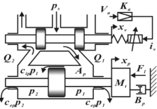
Fig. 1 represents the object hydraulic servo system in

(2)

this study. The main parts of the system are an electro-hydraulic servo valve, a servo cylinder and a mass(an inertia load). In the figure, p^s

is supply pressure, p¹

and p²

are pressure inside the cylinder chambers, Q and 1 Q are in-flowrate and out-flowrate 2

in the servo valve, and i_v is electric current given to the servo valve.

Fig. 1 Overview of the hydraulic system considered

2.2 Basic equations

Flowrate Q in the servo valve is described as1

l sv s l

Q K i p i p

 v i^v

v (1)

where ^K^sv



^^Q^ro^/



ⁱ^vr ^p^s

 

is a constant, Qro is flowrate when the rated current(ivivr) is supplied under no load(pl⁰) condition. Eq. (1) is effective when the flow in the valve is in a steady state.

When we consider the piston staying in the center point of the symmetric cylinder, the continuity equation in the cylinder is described as

4

p t l

l p tp l

c

dx V dp

Q A C p

dt  dt

  

(2)

where ^A^p is piston area, ^x^p is piston displacement, ^C^tp is leakage coefficient in the cylinder,  is effective ^e bulk modulus of oil in the cylinder, and ^V^t is total volume of oil in both chamber of the cylinder.

The equation of motion of the combined body of the piston and the load is shown as

2 2

p p

p l t p l

d x dx

A p M B F

dt dt

   (3)

where ^M^t is mass of the combined body, ^B^p is viscous friction coefficient, ^F^l is external force to the piston.

The spool position in the servo valve is approximated as

x_vk i_{v v} (4)

3. Feedback linearization-state feedback controller(FL-SFC)

This section describes the design procedure applying a feedback linearization technique to the object system to overcome the nonlinearities of the system. Differen- tiating the Eq. (3) with respect to time yields the following equation.

3 2

p p l p p

t t

d x A dp B d x dt M dt M dt

(5)

By substituting Eq. (2) and (3) to Eq. (5), we obtain the following equation.

3 2 2

3

4 4

p p e p e p p

l

t t t t t

d x A A B dx

dt M V Q M V M dt

 ^    ^

 

      (6)

² ²

4 _p _tp _e _p _p _p

l l

t t t t

A C A B B

p F

M V M M

  

   

 

Eq. (6) is rearranged as Eq. (7) by separating the terms including ^Q^l and the terms unrelated to ^Q^l.

3

3^p ^p, _l, _l ( ) _l

d x dx

f p F B x Q

dt dt

 

  

  (7)

where

2 2

( ^p, _l, )_l 4 ^p ^e ^p ^p

t t t

dx A B dx

f p F

dt M V M dt

    

 

      (8)

² ²

4 _p _tp _e _p _p _p

l l

t t t t

A C A B B

p F

M V M M



 

   

 

( ) 4 ^p ^e

t t

B x A M V

 

(9)

The nonlinearities can be excluded by using the following equation with regard to Ql.

(3)

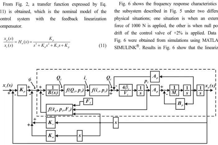
Fig. 3 Block diagram of the hydraulic control system using the FL-SFC

[the block surrounded with the dashed line can be simplified as ^{1/ s}³ by the feedback linearization]

, , ( )

p

l l l

Q f dx p F B x

 dt

  

   

 

  (10)

Thus, if the flowrate computed by the Eq. (10) is supplied to the system continuously, the condition

Fig. 2 Block diagram for the linearized system using FL-SFC

3 _p/ 3

d x dt  can be satisfied. Thereby, a linearized relationship between  and ^x^p is obtained. Then, a state feedback controller can be applied to the system, as shown in Fig. 2. And also the representative poles in the control system can be placed at the predetermined positions by adjusting the closed loop control gains.

From Fig. 2, a transfer function expressed by Eq.

(11) is obtained, which is the nominal model of the control system with the feedback linearization compensator.

3 2

( ) ( ) ( )

p p

n

r a p

x s K

x s H s s K s K s K

  v  (11)

Fig. 3 shows the block diagram of the control system with the FL-SFC. The state feedback control gains K

are computed by placing the representative poles at 38 24i

  (from the condition of _  rads   

for the representative poles), and another pole is placed at

 38 5on the real axis in the complex variable plane.

4. Sensitivity analysis of the system with the feedback linearization compensator

4.1 The object hydraulic control system

Fig. 4 shows the photograph of the object hydraulic control system. The values of physical parameters are listed in Table 1.

4.2 Sensitivity of the compensated system

Fig. 5 shows a simplified block diagram of the block surrounded with the dashed line in Fig. 3. ^{G s}^p^{( )} and

c( )

G s in the figure are the control object and the feedback linearization compensator part respectively.

Also, ① and ② depict null point drift in the control valve and external disturbances.

Fig. 6 shows the frequency response characteristics of the subsystem described in Fig. 5 under two different physical situations; one situation is when an external force of 1000 N is applied, the other is when null point drift of the control valve of +2% is applied. Data in Fig. 6 were obtained from simulations using MATLAB/

SIMULINK^Ⓡ. Results in Fig. 6 show that the linearized

(4)

model (1/ s³) can be affected on a large scale by the external force and the valve null point drift.

Table 2 shows the variation of poles of the object system in Fig. 3 under the variation of system parameters  , ^e ^B^p and ^M^t. The data were given from simulations using MATLAB/SIMULINKⓇ. In the simulation, the transfer functions between ^Q^l and ⁱ^v, and between ⁱ^v and ^Q^l in Fig. 3 were substituted as

‘1’. We can have a hint from the data in Table 2 on the fact that the control performances of the system shown in Fig. 3 might be affected severely under the variation of system parameters  , ^e ^B^p and Mt.

Fig. 4 Photo. of the experimental equipment

Table 1 The values of physical parameters in the object hydraulic system

[m ] : 0.000942

Ap ,

3 2

m / : 0

tp N/m C  s

 

  ,

N :15000

t m/s B  

 

  ,

9 2

N :1.4 10

e m

 ^ ^  , Fl

 

^{N : 0},^V^t ^^{m : 6 10}³^ ^ ^⁴, mA : 6

a V K  

 

  ,

V : 200

LT m K  

   , Mt

 

^{kg :118},

 

^{mA :15}

i_vr ,

3

9 2

m / : 8.0 10 mA N/m

s

K  s  ^

  

 

v ,

: 0.84

_v , _v



rad/s : 760



, ps^{[bar]: 35}

Fig. 5 Simplified block diagram of the block surrounded with the dashed line in Fig. 3

Fig. 6 Frequency response characteristics of the block surrounded with the dashed line in Fig. 3 with external force, with valve null point shift

5. Designing a disturbance observer In this section, the design process of the Feedback Linearization - State Feedback Controller with Disturbance Observer (FL-SFC-DOB) for the hydraulic servo system shall be described.

Fig. 7 shows a system with a disturbance observer.

( )

H s in the figure is the control system(including FL- SFC) shown in Fig. 3, and H sn^{( )} is the nominal model described by Eq. (11). ^{Q s}^{( )} is a filter for disturbance compensation, and ^{d s}^{( )} describes external disturbances or disturbance equivalence of system parameters’ variation.

Table 2 Poles of the object system shown in Fig. 3 under the variation of system parameters

pole 1 pole 2 pole 3 no variation －38+24i －38－24i －191

 : －50% e －31+30i －31－30i －104

 : ＋50% e －40+21i －40－21i －290 Bp : －50% －102+43i －102－43i －32 Bp : ＋50% －26+30i －26－30i －247 Mt : －90% －21+23i －21－23i －3990 Mt : ＋90% －22+85i －22－85i －27

Fig. 7 Application of a disturbance observer to the control system shown in Fig. 3

(5)

In this study, Umeno’s method⁷⁾ for disturbance compensation was applied to design ^{Q s}^{( )}. ^{Q s}^{( )} for the system was determined as Eq. (12), considering that the relative order between the numerator and the denominator of the system transfer function is 3.

3

( ) 3

( )

Q s s



 

 (12)

where  is a cut-off frequency.

6. Results of experiment and simulation

Experiments were done using the experimental system shown in Fig. 4. The values of the physical parameters of the experimental system are shown in Table 1. In all the experiments of this study, p was set to be 35 bar. s

For realizing digital control and signal measurements, a PC and MATLAB/RTWT⁸⁾ were used.

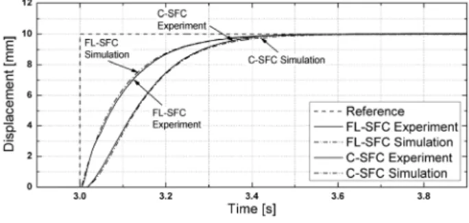
6.1 The results when「FL-SFC」applied

Fig. 8 shows the experimental and simulated results when a step input signal(0→10 mm) is given to the system with FL-SFC. In addition, responses of C-SFC(the Conventional State Feedback Controller applied to the hydraulic servo system) were included in the same figure to evaluate the results of FL-SFC objectively.

In designing C-SFC, a flow equation linearized in the operating point of the servo valve was used. Control gains for the C-SFC were obtained from the pole placement method. The representative poles for the C-SFC were placed at the same positions as ones for FL-SFC(designed in section 3) so as to enable an objective comparison of control performances of the

Fig. 8 Experimental and simulated results of the object system with C-SFC or with FL-SFC

systems with the FL-SFC and the C-SFC. And other poles were placed at  ^{38 5} on the real axis.

Fig. 8 shows the validity of the mathematical model of the control systems used in this study. In this figure, FL-SFC shows better response compared to C-SFC by reducing 17.1% in settling time(±2% basis for the final value of a step response).

6.2 The results when「FL-SFC-DOB」applied 6.2.1 Under external load

Fig. 10 shows the step responses of the control system under external load(Fig. 9) of ^W ^^{1000 N}. When FL-SFC was applied(Fig. 10 (a)), 0.4 mm steady- state error and undershoot response appeared. But, with FL-SFC-DOB application, the effects of the external load could be rejected clearly as shown in Fig. 10(b).

Fig. 9 Simplified schematic diagram of the load system in the object system

(a) when FL-SFC applied

(b) when FL-SFC-DOB( 200) applied Fig. 10 Experimental and simulated results of the

object system with external load ^W^^{1000 N}

(6)

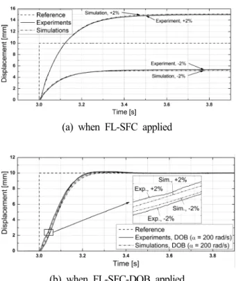
6.2.2 Under null point drift in the control valve In general, the allowable limit of null point drift in commercial servo valves⁹⁾ is said to be ±2%. Under the allowable limit value of null point drift, the control performances of the control system were investigated.

The null point drift in the servo valve was realized equivalently by shifting the null point of the servo amplifier output.

Fig. 11 shows the step responses of the control system under the null drift of ±2%. When FL-SFC was applied(Fig. 11 (a)), great steady state errors appeared, which was anticipated result by referring to Fig. 5. But, with the FL-SFC-DOB application, the effects of the null point drift could be removed and zero steady state error was realized.

6.2.3 Under the variations of ^M^t, ^B^p and  ^e The effects of the variations of the representative physical parameters Mt, ^B^p and  on the control ^e performances of the control system were investigated.

Step responses of the control system under the variation of Mt, ^B^p and  were shown in Fig. 12, 13 and 14.^e

(b) when FL-SFC-DOB applied

Fig. 11 Experimental and Simulated results of the object system under valve null point shift with +2%, -2%

(b) when FL-SFC-DOB applied

Fig. 12 Experimental and simulated results of the object system under ^M^t variation

(b) when FL-SFC-DOB( 200) applied Fig. 13 Simulated results of the object system

under ^B^pvariation

When FL-SFC was applied, change in control performances appeared according to the variation of

Mt, ^B^p and  . And, it was ascertained that, with e

(7)

FL-SFC-DOB application, the change in the control performances under the variation of Mt, ^B^p and  e

could be moderated in a great deal.

7. Conclusions

In this study, the control performance of a hydraulic servo system with a feedback linearization compensator and a disturbance observer was investigated. The focus of this study was set on the quantitative investigation of the effects(sensitivities) of system uncertainty on control performances of the hydraulic control system.

The sensitivity on the system uncertainty(changes in values of physical parameters of the control system, neutral point shift of the control valve, and disturbance input) of the hydraulic control system with a Feedback Linearization - State Feedback Controller(FL-SFC) which has not been covered in detail in the previous researches, was studied quantitatively by experiments and numerical simulations. As a result, it was confirmed that the system uncertainty may significantly affect the control performance in the hydraulic control system with FL-SFC.

(b) when FL-SFC-DOB( 200) applied Fig. 14 Simulated results of the object system

under  variation^e

Then, a Feedback Linearization - State Feedback Controller with Disturbance Observer (FL-SFC-DOB) was designed for the hydraulic servo system. From the experiments and numerical simulations, it was confirmed the control with FL-SFC-DOB can guarantee excellent and robust control performance under the existence of system uncertainty and external disturbances.

References

1) I. Iwan et al., “Controller Design for a Nozzle-flapper Type Servo Valve with Electric Position Sensor”, Journal of Drive and Control, Vol.16, No.1, pp.29~35, 2019.

2) S. D. Kim, J. E. Lee and D. Y. Shin, "A Study on the Phase Bandwidth Frequency of a Directional Control Valve Based on the Hydraulic Line Pressure", Journal of Drive and Control, Vol.15, No.4, pp.1-10, 2018.

3) G. H. Jun and K. K. Ahn, "Extended-State- Observer-Based Nonlinear Servo Control of An Electro-Hydrostatic Actuator", Journal of Drive and Control, Vol.14, No.4, pp.61-70, 2017.

4) G. A. Sohl and J. E. Borrow, “Experiments and Simulations on the Nonlinear Control of a Hydraulic Servo system”, IEEE Transactions on Control Systems Technology, Vol. 7, No. 2, pp. 238~247, 1999.

5) I. Tunay, E. Y. Rodin and , A. A. Beck, “Modeling and Robust Control Design for Aircraft Brake Hydraulics”, IEEE Transactions on Control Systems Technology, Vol.9, No.2, pp.319~329, 2001.

6) L. D. Re and A. Isidori, “Performance Enhancement of Nonlinear Drives by Feedback Linearization of Linear-Bilinear Cascade Models”, IEEE Transactions on Control Systems Technology, Vol.3, No.3, pp.

299~308, 1995.

7) T. Umeno, T. Kaneko and Y. Hori, “Robust Servo system Design with two Degrees of Freedom and its Application to Novel Motion Control of Robot Manipulators”, IEEE Transactions on Industrial Electronics, Vol.40, No.5, pp.473-485, 1993.

8) The MathWorks, Inc., Real-Time Windows Target^TM User's Guide, 2008.

9) https://www.moog.com/literature/ICD/Moog-ServoValv es-G761_761Series-Catalog-en.pdf