The Estimating Equations Induced from the Minimum Dstance Estimation

(1)

2003, Vol. 14, No.3 pp. 687∼696

The Estimating Equations Induced from the Minimum Dstance Estimation¹⁾

Ro Jin Pak²⁾

Abstract

This article presents a new family of the estimating functions related with minimum distance estimations, and discusses its relationship to the family of the minimum density power divergence estimating equations.

Two representative minimum distance estimations; the minimum _L₂ distance estimation and the minimum Hellinger distance estimation are studied in the light of the theory of estimating equations. Despite of the desirable properties of minimum distance estimations, they are not widely used by general researchers, because theories related with them are complex and are hard to be computationally implemented in real problems.

Hopefully, this article would be a help for understanding the minimum distance estimations better.

Keywords : Density power divergence; estimating equations; Hellinger distance

1. Background and Motivation

In most of the previous works, the minimum distance estimation (MDE) has been studied by focusing on estimators, but in this article we focus rather on estimating equations which produce estimators. The theory of estimating equations has been well established since Godambe (1960), and has been a hot topic in the field of estimation for a while (Godambe and Thomson (1974), Godambe (1976)).

By investigating the MDE in the estimating equation's point of view, we are

1) The present research was conducted by the research fund of Dankook University in 2002.

2) Associate Professor, Department of Computer Sciences and Statistics, Dankook University, Seoul, Korea, 140-714.

E-mail : [email protected]

(2)

given a new tool to tackle the MDE estimation to enhance its generality and applicability. In the section 2.1 we provide a general form of estimating equations based on MDE covering both the minimum Hellinger distance estimation (MHD estimation) and the minimum L2 distance estimation (ML2D estimation). The MHD estimation (section 2.2) and the ML2D estimation (section 2.3) are studied one by one in the light of the theories of estimating equations. We also show that the proposed estimating equations turn out to be as same as those obtained by minimizing the density power divergence (Basu et al., 1998).

2. Properties of estimation equations by minimum distance estimations

2.1 General Form

Given an i.i.d. random sample, X1,X₂,…,X_n, having a density fθ(x), let f_n(x) be a density estimator for f_θ(x) such as

f_n(x) = 1

n ∑ _h¹ ^k

(

^{x - X}^h ⁱ

)

^,

where k(⋅) is a kernel and h is a bandwidth. Define a smoothed density as f^*_θ(x)= ⌠⌡f ^θ(x-y)k(y) dy and consider a family of distances between a smoothed density and a corresponding density estimator indexed by a parameter β as

{

^⌠^{⌡( f}^1/βⁿ ^{(x) - f}^{* 1/β}^θ ^{(x) )}²^{dx, 1≤β≤2}

}

The distance we define here is differ from an usual distance by means of using a smoothed density in place of a density itself. Since E[ f_n(x)]= f^*_θ(x), it really helps us to reduce fair amount of mathematical complexity in theories.

The Hellinger distance ( β=2) and the squared distance (or L2 distance ( β=1)) are members of this family. The minimum distance estimator ( θ ˆ) is defined as a solution to

∇_θ⌠

⌡(f^1/βⁿ (x) - f^{* 1/β}_θ (x) )²dx =- 2 ⌠⌡( f^1/βⁿ (x) - f^{* 1/β}_θ (x)) 1 β

∇_θf^*_θ(x) f* ( 1- 1/β)

θ (x) dx = 0, where ∇θ represents a derivative w. r. t. θ.

Theorem 2.1. For 1≤β≤2

⌠ (1)

⌡( f^1/βⁿ (x)-f^{* 1/β}_θ (x)) 1 β

∇_θf^*_θ(x) f* ( 1 - 1/β)

θ (x) dx

(3)

can be reduced to 1 β ⌠

⌡( fⁿ(x)-f^*_θ(x)) f* ( - 1 +1/β)

θ (x) ∇_θf^*_θ(x)

f* ( 1 - 1/β)

θ (x) dx.

Proof. Consider the following series expansion;

(2) f^1/β_n (x) - f^{* 1/β}_θ (x) = 1

β ( f_n(x)-f^*_θ(x)) f* ( - 1 +1/β)

θ (x)

+ 1

2β ( - 1 + 1

β )( f_n(x)-f^*_θ(x))²f* ( - 2 + 1/β)( x) θ

+o( ( f_n(x)-f^*_θ(x))³).

and put (2) into (1) then the second term in the resulting integral,

⌠⌡ 1

2β ( - 1 + 1

β )( f_n(x)-f^*_θ(x))²f* ( - 2 + 1/β)

θ (x) ∇_θf^*_θ(x)

f* ( 1- 1/β)

θ (x) dx

= 1

2β( - 1 + 1

β ) ⌠⌡

(

^fⁿ^(x)-f^f^*^θ^(x)^*^θ^(x)

)

²^f* ( - 1 + 2/β)

θ (x) ∇_θf^*_θ(x) dx

→ 0 in probability as n→∞,

since both f_n(x)-f^*_θ(x) /f^*_θ(x)→ 0 as n→∞ and that f* ( - 1 + 2/β)

θ (x)∇_θf^*_θ(x) is bounded for -1 +2/β≥0. Similarly, we can show that the higher order terms go to 0 in probability. □

Also, we can rewrite the second integral in Theorem 2.1, 1

β

⌠⌡( fⁿ(x)-f^*_θ(x)) f* ( - 1 +1/β)

θ (x) ∇_θf^*_θ(x)

f* ( 1 - 1/β)

θ (x) dx

as

1

nβ ∑^⌠_⌡

{

^h¹ ^k

(

^{x - X}^h ⁱ

)

^{- f}^*^θ^(x)

}

^f* ( - 1 + 2/β)

θ (x) ∇_θlog f^*_θ(x) dx, which leads to the following definition.

Definition 2.1. Define a general form of the estimating equation for 1≤β≤2 as

g( y) = ⌠⌡

{

¹^h ^k

(

^{x - y}^h

)

^{- f}^*^θ^(x)

}

^f* ( - 1 +2/β) (3)

θ (x)∇_θlog f^*_θ(x) dx.

If β = 2 then (3) becomes (5), which is an estimating equation producing efficient but non-robust estimators (section 2.2). If β = 1 then (3) becomes the estimating equation (6), which is an M-estimating equation producing a robust but not fully efficient estimator (section 2.3). □

(4)

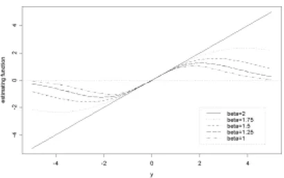
Figure 1. Estimating equations for μ .

Figure 1 displays the estimating equation g(y) for different values of β, when a kernel is Gaussian and a density is N(μ,σ²) with σ and h being fixed. When β is 2, g( y) = y, which is known to produce a non-robust but fully efficient estimator (so called, least squares estimator / MLE under Normal distribution).

For 1≤β < 2, g( y) displays redescending nature producing robust but not fully efficient estimators. It can be claimed that the value of β controls trade-off between efficiency and robustness.

Remark 2.1. The estimating equation based on a density power divergence (Basu, et al., 1998) can be reproduced by the estimating equation (3) as follows;

Consider the first part in (3). Let z = ( x - y)/h and do Taylor Series expansion about y, then we have

⌠⌡ 1

h k

(

^{x - y}^h

)

^f* ( - 1 + 2/β)

θ (x) ∇_θlog f^*_θ(x) dx

= ⌠⌡k( z)f

* ( - 1 + 2/β)

θ (y+hz) ∇_θlog f^*_θ(y+hz) dz

= ⌠⌡[^{k( z) f}* ( - 1 + 2/β)

θ (y) + hz∇yf* ( - 1 + 2/β)

θ (y)+ …][^∇^θ^{log f}^*^θ^{(y) + hz∇}^y^∇^θ^{log f}^*^θ^{(y) + …}]^dz

= f* ( - 1 + 2/β)

θ (y) ∇_θlog f^*_θ(y) ⌠⌡k( z)dz + o( h)

= f* ( - 1 + 2/β)

θ (y) ∇_θlog f^*_θ(y) + o( h).

Hence, g(y) in Definition 2.1 turns out

(5)

f* ( - 1 + 2/β)

θ (y) ∇_θlog f^*_θ(y) + ⌠⌡f^{* ( 2/β)}^θ (x)∇_θlog f^*_θ(x) dx + o( h).

Since f^*_θ(x) →f_θ(x) as h→0, then g( y) becomes u_θ(y)f( - 1 + 2/β)

θ (y) - ⌠⌡u^θ(y) f^2/β_θ (y)dy,

where uθ(y) is the maximum likelihood score function. The above equation turns out to be as same as the ψ( y,θ) (Basu, et al., 1998) with 2/β = 1+α;

ψ( y,θ) = u_θ(y)f^α_θ(y) - ⌠⌡u^θ(y)f^{1 + α}_θ (y)dy.

Basu, et al. (1998) claimed that the degree of compromise between efficiency and robustness would be controlled by the tuning parameter α. Choices of α near zero, i. e. β near two, are known to afford considerable robustness while retaining efficiency close to that of maximum likelihood. □

2.2 Hellinger Distance : _β=2

The Minimum Hellinger distance estimator based on Basu and Lindsay (1994) is a solution to

∇_θ⌠ (4)

⌡(f^1/2ⁿ (x) - f^{* 1/2}_θ (x) )²dx =- 2 ⌠⌡( f^1/2ⁿ (x) - f^{* 1/2}_θ (x)) ∇_θf^*_θ(x)

f^{* 1/2}_θ (x) dx =0.

For b≥0, a > 0 we have an algebraic identity

b^1/2-a^1/2= ( b - a)/2a^1/2- ( b - a)²/[ 2a^1/2(b ^1/2+a^1/2)²].

By combining this identity with (4), we have

⌠⌡( f^1/2ⁿ (x) - f^{* 1/2}_θ (x)) ∇_θf^*_θ(x)

f^{* 1/2}_θ (x) dx = 1 2 ⌠

⌡( fⁿ(x) - f^*_θ(x)) ∇_θf^*_θ(x)

f^*_θ(x) dx + R_n, where

R_n=- ( f_n(x) - f^*_θ(x))²/[2f^{* 1/2}_θ (x) ( f^1/2_n (x) + f^{* 1/2}_θ (x))²].

Suppose R_n= o_p(1), which is in fact true by Beran (1977), then

⌠⌡( f^1/2ⁿ (x) - f^{* 1/2}_θ (x)) ∇ _θf^*_θ(x)

f^{* 1/2}_θ (x) dx and 1 2

⌠⌡( fⁿ(x) - f^*_θ(x)) ∇_θf^*_θ(x) f^*_θ(x) dx are asymptotically equivalent, and we have

⌠

⌡( fⁿ(x) - f^*_θ(x)) ∇_θf^*_θ(x)

f^*_θ(x) dx = 1

n ∑^⌠_⌡ _h¹ ^k

(

^{x - X}^h ⁱ

)

^∇ ^θ^{log f}^*^θ^{(x) dx.}

Remark 2.2. The estimating equation based on the Hellinger distance,

(6)

g( y) = ⌠⌡ 1 (5)

h k

(

^{x - y}^h

)

^∇^θ^{log f}^*^θ^{(x) dx}

= ⌠⌡

{

¹h k

(

^{x - y}h

)

^{- f}^*^θ^(x)

}

^∇^θ^{log f}^*^θ^{(x) dx,}

which is the g(y) in Definition 2.1 with β = 2, is an unbiased optimal estimating equation when h→0. Proofs are in Appendix. □ Example 2.1. Suppose that a kernel is Gaussian, and that the model density is N( μ,σ²), then f^*_θ(x) is N( μ,h²+ σ²). Therefore, we have

g( y) = ⌠⌡ 1

h k

(

^{x - y}^h

)

^∇^θ^{log f}^*^θ^{(x) dx =}

[

( y - μ)/( h²+ σ²)

]

( - h²- σ²+(y- μ)²)/2( h²+ σ²)² which is a vector of score functions of N(μ,σ²), which is unbiased and optimal, in case of h→0. □

2.3 L₂ Distance : β=1

The minimum L2 distance estimator is solution to

∇_θ⌠

⌡(fⁿ(x) - f^*_θ(x))²dx =- 2 ⌠⌡( fⁿ(x) - f^*_θ(x)) ∇_θf^*_θ(x) dx = 0, and we have

⌠⌡( fⁿ(x) - f^*_θ(x))∇_θf^*_θ(x) dx =∑^⌠_⌡

{

^h¹ ^k

(

^{x - X}^h ⁱ

)

^{- f}^*^θ^(x)

}

^∇^θ^f^*^θ^{(x) dx.}

Remark 2.3. The estimating equation based on minimization of L₂ distance as g( y) = ⌠⌡

{

^h¹ ^k

(

^{x - y}^h

)

^{- f}^*^θ^(x)

}

^f^*^θ^{(x) ∇}^θ^{log f}^*^θ^{(x) dx.} (6)

which is the g( y) in Definition 2.1 with β = 1, is a robust estimating function, but asymptotic optimality is not naturally given as shown as follows:

Define the matrices J_g= E[ gg^T] and M_g= E[∂ g/∂θ], and then the efficiency matrix is Eff ( g) = M^{- 1}_g J_g(M^{- 1}_g )^T.

The expectation of the first derivative of the estimating equation in (6), M_g = E

[

^⌠^⌡

{

h¹ k

(

^{x - y}h

)

^{- f}^*^θ^(x)

}

^∇²^θ^f^*^θ^{(x) dx - ⌠}^⌡∇^θ^f^*^θ^{(x) ∇}^θ^f^*^θ^(x)dx

]

= ⌠⌡

[

^E

{

h¹ k

(

^{x - y}h

)}

^{- f}^*^θ^(x)

]

^∇²^θ^f^*^θ^{(x) dx - ⌠}^⌡∇^θ^f^*^θ^{(x) ∇}^θ^f^*^θ^{(x) dx}

→ 0 - ⌠⌡∇^θf²_θ(x) dx,

which is not equal to -I( θ) ( = E[ ∇_θlog f^*_θ(x)²]) as h→0. □ Example 2.2. Suppose that a kernel is Gaussian, and that f is N(μ,σ²). After

(7)

dropping unnecessary constant factors, we have g( y) =

ꀎ

ꀚ

︳︳

ꀏ

ꀛ

︳︳

︳︳ ( y - μ) exp

{

^2(2h^{- ( y- μ)}²^+σ²²⁾

}

{

^{- 1+} ^{( y - μ)}^2h²^+σ²²

}

^exp

{

^2(2h^{- ( y- μ)}²^+σ²²⁾

}

⁺

{

^2h^2h²²^+2σ^{+ σ}²²

}

^3/2

.

We can not attain optimal asymptotic efficiency with g( y) even if h→0, because g(y) is far from the score function of the normal density, due to the factor exp (⋅). □

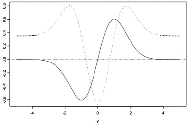
Figure 2. Estimating equations for μ (solid) and σ²(dotted).

y

-4 -2 0 2 4

-0.6-0.4-0.20.00.20.40.60.8

y

-4 -2 0 2 4

-0.6-0.4-0.20.00.20.40.60.8

Figure 2 displays estimating equations given in Example 2.2 with h and σ being fixed. They clearly show redescending nature of M-estimating functions.

Each equation is of redescending types of M-estimating equations producing robust estimators for μ and σ², respectively. Robustness of the estimators by the above estimating equation g(y) is ensured, while losing some efficiency.

Remark 2.4. If we redefine g_s(y) = g( y) E[ ∂g( y)/∂θ]^{- 1} then we have E[ g_s(y)] = 0, since E[ h^{- 1}k {h^{- 1}(x-y) }] = f^*_θ(x). Therefore, g _s(y) is an unbiased estimating equation. Optimality is trivial because the standardized estimating equation is the optimal estimating equation, among unbiased estimating equations (Godambe, 1960). □

(8)

2.4 Optimality for a bandwidth

As we can notice from Example 2.1 and 2.2, the estimators based on g(y) are M-estimators. Recall that an M-estimator is optimal V-robust (Hampel et al., 1986) when it minimizes V( ψ,F) for a given upper bound on κ ^*(ψ, F)(

change-of-variance sensitivity) where ψ is an M-estimating equation. Hall and Marron (1991) have shown that the best possible relative rate of convergence to the optimum for the data driven bandwidth selector is n^{- 1/2}. Moreover, Fan and Marron (1992) have obtained the 'Fisher like' lower bound of the relative errors of bandwidth selector, which is given by

σ²(f) = 4 25

ꀎ ꀚ

︳︳

⌠⌡( f

( 4))²f { ⌠⌡( f '')²}²- 1

ꀏ ꀛ

︳︳

︳︳.

Kim, Park and Marron (1994) give bandwidth selectors, h, which achieve the above best rate and best constant in the sense that for a fixed bandwidth h0

n^1/2(h/h ₀-1) ⇒N( 0,σ²(f)).

Since V(g(y;h),F) is in terms of h, we can discuss the optimality of h in the light of density estimation. Expand the asymptotic variance of an estimating equation in terms of the bandwidth for a fixed bandwidth h0;

n {V( g( y;h),F) - V( g( y;h₀),F) } = ( h - h₀)V '( g( y;h),F)|_{h = h}₀ + 1

2( h - h₀)²V ''(g( y;h),F)| _{h = h}₀+ ….

Suppose we neglect higher terms except the first order term, we have n ^1/2h^{- 1}₀ V(g(y;h),F)-V( g( y;h₀),F) ≅

n^1/2(h/h ₀- 1)V '( g( y;h),F)|_{h = h}₀ ⇒ N( 0,σ²(f) V '²(g(y;h),F )|_{h = h}₀).

The variance is in the form of `constant times σ²(f)', so that optimality of h in our problem can be consider in the same manner as we deal with the optimality in density estimation. Therefore, for example, the plug-in type bandwidth proposed by Sheather and Jones (1991) would be a good optimal choice for h.

3. Conclusions

A new family of the estimating equations indexed by a parameter β covers various estimating equations producing robust and/or efficient estimators. The larger the β is, the more we get efficiency, and the smaller the β is, the more

(9)

we get robustness. The two representative minimum distance estimations; the minimum L2 distance estimation and the minimum Hellinger distance estimation are studied by the proposed family of the estimating equations. The relation between the minimum distance estimation and the estimation by minimizing a density power divergence by Basu, et al. (1998) is presented. We hope that this article would be a little help for people to understand minimum distance methodology.

4. Appendix

First, the expectation of the estimating equation (5),

E[ g( y)] = E

[

^⌠^⌡ h¹ k

(

^{x - y}h

)

^∇^θ^{log f}^*^θ^{(x) dx}

]

^{= ⌠}^⌡E

[

h¹ k

(

^{x - y}h

)]

^∇^θ^{log f}^*^θ^{(x) dx}

= ⌠⌡f^*^θ(x) ∇_θf^*_θ(x)

f^*_θ(x) dx = ⌠⌡f^*^θ(x) ∇_θlog f^*_θ(x) dx

= ⌠⌡∇^θf^*_θ(x)dx = ∇_θ⌠

⌡f^*^θ(x) dx = 0, which implies that the estimation function is unbiased.

Furthermore, since we have f^*_θ(x) →f_θ(x) as h→0 M_g = E[ ∂g/∂θ] = E

[

^⌠^⌡ ^h¹ ^k

(

^{x - y}^h

)

^∇²^θ^{log f}^*^θ^{(x) dx}

]

= ⌠⌡f^*^θ(x) ∇²_θlog f^*_θ(x) dx = ⌠⌡f^*^θ(x)

(

^∇²^θ^f^*^θ^{(x) f}^*^θ^{(x) - ( ∇}^f^{* 2}^θ^(x) ^θ^f^*^θ^(x))²

)

^dx

= ⌠⌡∇²^θf^*_θ(x)dx - ⌠⌡

(

^∇^f^θ^*^θ^f^(x)^*^θ^(x)

)

²^f^*^θ(x)dx = 0 - ⌠⌡

(

^∇^f^θ^*^θ^f^(x)^*^θ^(x)

)

²^f^*^θ^(x)dx

→ - ⌠⌡

(

^∇^f^θ^θ^f^(x)^θ^(x)

)

²^f^θ(x) dx =- E[( ∇_θlog f_θ(x) )²]= - I( θ) as h→0.

Hence, if J_g= E[ gg^T]→I( θ) as h→0, then Eff ( g) →I^{- 1}(θ), so that g( y) becomes an unbiased optimal estimating equation. □

References

1. Basu, A. and Lindsay, B. G. (1994). Minimum disparity estimation for continuous models: efficiency, distributions and robustness, Annals of the Institute of Statistica Mathematic, 46, 683-705.

2. Basu, A., Harris, I. R., Hjort, N. L. and Jones, M. C. (1998). Robust

(10)

and efficient estimation by minimizing a density power divergence, Biometrika, 85, 549-559.

3. Beran, R. J. (1977). Minimum Hellinger distance estimates for parametric models, Annals of Statistics, 5, 445-463.

4. Fan, J. and Marron, J. S. (1992). On optimal data-based bandwidth selection in kernel density estimation, Biometrika, 78, 263-269.

5. Godambe, V. P. (1960). An optimum property of regular maximum likelihood estimation, Annals of Mathematical Statistics, 31, 1208-1212.

6. Godambe, V. P. (1976). Conditional likelihood and unconditional optimum estimating equations, Biometrika, 63, 277-284.

7. Godambe, V. P. and Thomson, M. E. (1974). Estimating equations in the presence of a nuisance parameter, Annals of Statistics, 2, 568-571.

8. Hampel, F. R., Ronchetti, E. M., Rousseeuw, P. J. and Stahel, W. A.

(1986). Robust Statistics, the Approach Based on Influence Functions, John Wiley & Sons, New York.

9. Hall, P. and Marron, J. S. (1991). Lower bounds for bandwidth selection in density estimation, Probability Theory and Related Fields, 90, 149-17.

10. Kim, W. C., Park, B. U. and Marron, J. S. (1994). Asymptotically best bandwidth selectors in kernel density estimation, Statistics and

Probability Letters, 19, 119-127.

11. Sheather, S. J. and Jones, M. C. (1991). A reliable data-based

bandwidth selection method for kernel density estimation, Journals of the Royal Statistical Society, Series. B, 53, 683-690.

[ received date : Mar. 2003, accepted date : Jul. 2003 ]