An Efficient Identification Algorithm in a Low SNR Channel

접수일자 : 2014. 02. 11 심사완료일자 : 2014. 03. 02 게재확정일자 : 2014. 03. 20

* Corresponding Author Juphil Cho(E-mail: [email protected], Tel: +82-63-469-4749)

Department of Radiocommunication Engineering, Kunsan National University, Kunsan 573-701, Korea

Open Access http://dx.doi.org/10.6109/jkiice.2014.18.4.790

This is an Open Access article distributed under the terms of the Creative Commons Attribution Non-Commercial License(http://creativecommons.org/li-censes/

한국정보통신학회논문지(J. Korea Inst. Inf. Commun. Eng.) Vol. 18, No. 4 : 790~796 Apr. 2014

저 SNR을 갖는 채널에서 효율적인 인식 알고리즘

황지원¹ · 조주필^2*

An Efficient Identification Algorithm in a Low SNR Channel

Jeewon Hwang ¹ · Juphil Cho ^2*

1

Department of Information Technology, Chonbuk National University, Jeonju 561-756, Korea

2*

Department of Radiocommunication Engineering, Kunsan National University, Kunsan 573-701, Korea

요약

통신채널의 인식문제는 현재 이론적 부분과 실제 관점 부분의 문제점을 가지고 있다. 최근에 이 문제를 해결키 위 해 제안된 기법들은 안테나 구조와 시간 오버샘플링에 의해 유도된 다이버시티를 이용하고 있다. 이 방법은 선형 제

한조건을 가진 적응필터를 이용하고 있다 . 본 논문에서는 값 분할에 근거한 기법이 제안되었다. 수신신호 상관행렬

의 최소 단일값에 의한 단일벡터는 채널 임펄스 응답을 포함하며 상기 문제를 해결키 위한 적응 알고리즘을 보인다.

제안된 기법은 기존 기법의 성능보다 우수함을 알 수 있다 .

ABSTRACT

Identification of communication channels is a problem of important current theoretical and practical concerns.

Recently proposed solutions for this problem exploit the diversity induced by antenna array or time oversampling. The method resorts to an adaptive filter with a linear constraint. In this paper, an approach is proposed that is based on decomposition. Indeed, the eigenvector corresponding to the minimum eigenvalue of the covariance matrix of the received signals contains the channel impulse response. And we present an adaptive algorithm to solve this problem.

Proposed technique shows the better performance than one of existing algorithms .

키워드 : 신호대잡음비, 채널, 인식, 상관

Key word : SNR, channel, identification, covariance.

Communication Engineering

Ⅰ. INTRODUCTION

In HOS-based methods, because the performance index as the optimization criterion is nonlinear with respect to estimation parameters and these methods require a large amount of data samples. These methods have the disadvantage that their computational complexity may be large. See, for example, [1] and references therein. Since the seminal work by Tong et al. the problem of estimating the channel response of multiple FIR channel driven by an unknown input symbol has interested many researchers in signal processing and communication fields. This is achieved by exploiting assumed cyclostationary properties, induced by oversampling or antenna array at the receiver part[1,2].

The basic blind channel identification problem involves a channel model where only the observation signal is available for processing in the identification channel.

Earlier blind channel identification approaches mostly depend on higher order statistics (HOS), because the second order statistics (SOS) does not contain phase information for stationary signal[3-4]. Most communi- cation channels are time-varying in practice. Therefore, the algorithms should be able to track the change of the channel impulse response. Moreover, in a fast fading channel, the multipath channels in wireless communications vary rapidly, and we only have a few data samples corresponding to the same channel characteristics. Blind channel identification technique has been developed in adaptive algorithm based on vector-correlation method [8,9,11]. But most algorithms neglected the effect of channel noise.

Most notations are standard: vectors and matrices are boldface small and capital letters, respectively; the matrix transpose, the complex conjugate, the Hermitian, and convolution are denoted by ⋅ ^ , ⋅ ^ , ⋅ ^ and ⊗, respectively;  _ is the  ×  identity matrix;

  ⋅ is the statistical expectation.

This paper is organized as follows. In section II, we review the basic assumption and identification issues.

And the existing adaptive algorithms of the block LS

methods are described also. A novel blind channel identification technique based on eigenvlaue decom- position and adaptive implementation are proposed in section III. Simulation results with real measured channel are performed in section IV. Section V concludes our results.

Ⅱ. Basic Assumption and Issues

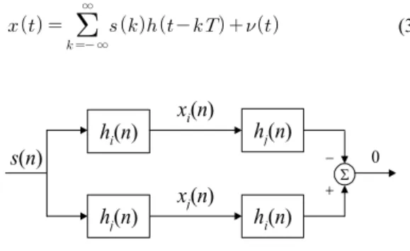
In this paper, consider a special case, when the channel output is two times oversampled or there are two antennas at the receiver, this is equivalent to two channel representation (   ). From the Fig. 1, in the absence of noise, it is apparent that the output of each subchannel is

 _    _ ⊗

 _    _ ⊗ (1)

Then

 _ ⊗ _    _ ⊗ _ ⊗ 

  _ ⊗ _ ⊗ 

  _ ⊗ _ 

(2)

Let  be the signal at the output of a noisy channel

  

  ∞

∞

        (3)

h _i

h _j

s(n)

h _j

n

h _i

n

x _i

x _j

− 0

+

그림 1. 두 서브채널간 상관관계

Fig. 1 The cross relation between two subchannels

s(n)

v

a

...

h

v

a

v

a

x

x

x

h

h

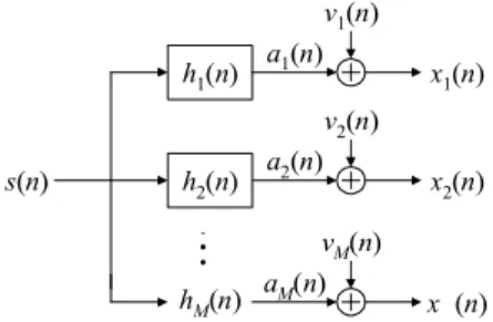
그림 2. M 서브채널을 갖는 등가 SIMO 모델

Fig. 2 Equivalent SIMO model with M subchannels

where  denotes the transmitted symbol at time

  ,  denotes the continuous-time channel impulse response, and  is additive noise. As shown in [3], the single channel system can be considered as the multichannel system by the sampling the received signal at a rate faster than the input symbol rate. The source signal  then passes through  equivalent symbol rate linear filters. And as shown in Fig. 2,  _ 

denotes the output from the ith channel with the noisy FIR channel impulse response { _ }, which is driven by the same input . Clearly, for linearly modulated communication signals,  _ ,  _ , ,  _ , and  _  are related as follows

 _   

  



 _      _ 

  _    _     ⋯ 

(4)

where  is the maximum order of the  channels.

The blind identification problem can be stated as follows: Given the observation of channel output { _ ,   ⋯  ;    ⋯  }, determine the channels and further recover the input signals {}.

As in classical system identification problems, certain conditions about the channel and the source must be satisfied to ensured identifiability. We assume the following throughout in this paper about the channel and source conditions.

A1) Subchannels do not share common zeros, or in other words, they are coprime.

A2) The noise  is zero mean, white with known covariance, no cochannel correlation, and uncorrelated with source signal.

A3) The channel has known order  .

The assumption that  is known may be practical. To address this problem, there are three approaches[5].

First, channel order detection and parameter estimation can be performed separately. Second, some statistical subspace methods require only upper bound of  . Third, channel order detection and parameter estimation can be performed jointly.

Ⅲ. Proposed Scheme

As described in [5], to avoid the trivial solution to minimization problem a proper condition must be selected. In this section, a new approach is proposed that is based on eigenvalue decomposition. Indeed, the eigenvector corresponding to the minimum eigenvalue of the covariance matrix of the received signals contains the channel impulse response. This approach is based on the unit norm constraint that is apart from the linear constraint introduced in the previous section[6].

A. Concept of the Proposed Scheme

Number equations consecutively with equation numbers in parentheses flush with the right margin, as in (1). We assume that the channel is linear and time invariant within small time interval; therefore, we have the following relation as described in (4)

x _ ^ h _   _ ^ h _ (5)

where

x _    _ ⋯  _      ^      (6)

and the channel impulse response vector of length L

are defined as

h _   _  _ ⋯  _{  }  ^      (7)

The covariance matrix of the two received signals is given by

R _x  



^



R _xx R _xx

R _xx R _xx (8)

Consider the 2L´1 vector as follows:

h  





^

 h _

 h _ (9)

From (5) and (8), it can be seen that R

h=0, which means that the vector h is the eigenvector of the covariance matrix R

corresponding to the eigenvalue 0.

Moreover, if the two channel impulse response h

and h

have no common zeros and the autocorrelation matrix of the source signal  is full rank, which is assumed in the rest of this paper, the covariance matrix R

has one and only one eigenvalue equal to zero. Consider the noisy channel case as described in (2) and let M=2. It follows from (1) that

x ^ h   _{  } ^{         } _{  }  ^{        }

 

  



 _ ^    _   

  



 _ ^    _ 

 v ^ h

(10) where x  x _ ^  x _ ^  ^ and

v  v _ ^  v _ ^  ^ .

If the correlation matrix of the vector x(n) is denoted by R

, a direct of conclusion of (10) will be

R _x h   xx ^ h  xv ^ h

  vv ^ h R _v h  _ ^ h (11)

We note from (11) that h is the eigenvector of the correlation matrix R

and  _ ^ is the corresponding

eigenvector of R

. The knowledge of  _ ^ can be obtained as a by product if wanted.

 _ ^   h ^H h h ^H R _x h

(12)

B. Adaptive Algorithm

In practice, it is simple to estimate iteratively the eigenvector corresponding to the minimum eigenvalue of R

, by using an algorithm similar to the Frost algorithm that is a simple constrained LMS algorithm [7].

Minimizing the quantity h ^ R _x h with respect to h and subject to ||h||

=h

h=1 will give us the optimum weight h

.

Let us define the error signal

    ║h║

h ^ x (13)

where x  x _ ^  x _ ^  ^ . Note that minimizing the mean square value of e(n) is equivalent to solving the above eigenvalue problem. Taking the gradient of e(n) with respect to h(n) gives

∇    ║h║

  x    ║h║

h  ⁽¹⁴⁾

and we obtain the gradient-descent constrained LMS algorithm:

h    h   ^ ∇  (15)

where , the adaptation step-size, is a positive constant.

Substituting (13) and (14) into (15) gives

h    h   ∥h∥

 ⋅

 ^{xx   } ∥h∥

h   ^  ∥h∥

h  ⁽¹⁶⁾

and taking statistical expectation after convergence, we get

R _x  ∥h∞∥

h∞     ^  ∥h∞∥

h∞ (17)

which is what is desired: the eigenvector h∞

corresponding to the smallest eigenvalue E[|e(n)|

] of the covariance matrix R

.

In practice, it is advantageous to use the following adaptation scheme

h    

h   ^ ∇

h   ^ ∇

(18)

The algorithm (18) presented above is very general to find the eigenvector corresponding to the smallest eigenvalue of any matrix R

. If the smallest eigenvalue is equal to zero, which is the case here, the algorithm can be simplified as follows:

   h ^ x (19)

and

h    

h   ^ x

h   ^ x

(20)

Ⅳ. Simulation Results

Computer simulations were conducted to evaluate the performance of the proposed algorithm in comparison with existing algorithms. In all the simulations, two channel SIMO model is assumed. This means two times oversampling or two sensors at the receiver in real situation. The input signal is 4-QAM. For simplicity of comparison, we assumed that the channel order L is known. The performance index is achieved by examination the root mean square error (RMSE) that is defined as [4].

RMSE  ∥h∥ ^

  ^{  } 

 

  



∥

^{ h}   h

^{ (21)}

where  _ is number of Monte Carlo trials, and  h _ is the estimate of the channels from the ith trial.

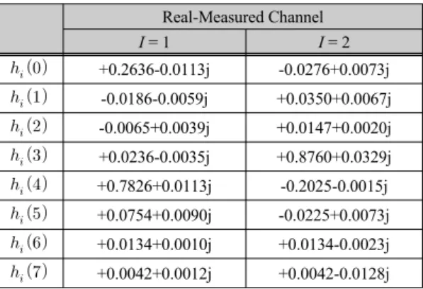
We used real-measured microwave channel. The shortened length-16 version of an empirically measured T/2-spaced digital microwave radio channel (M=2) with 230 taps, which we truncated to obtain a channel with L=7. The Microwave channel chan1.mat is founded at http://spib.rice.edu/spib/ microwave.html.

Real-Measured Channel

I = 1 I = 2

_ +0.2636-0.0113j -0.0276+0.0073j

_ -0.0186-0.0059j +0.0350+0.0067j

_ -0.0065+0.0039j +0.0147+0.0020j

_ +0.0236-0.0035j +0.8760+0.0329j

_ +0.7826+0.0113j -0.2025-0.0015j

_ +0.0754+0.0090j -0.0225+0.0073j

_ +0.0134+0.0010j +0.0134-0.0023j

_ +0.0042+0.0012j +0.0042-0.0128j 표 1. 채널 계수

Table. 1 Channel Coefficients

The shortened version is derived by linear decimation of the FFT of the full-length T/2-spaced impulse response and taking the IFFT of the decimated version (see [10] for more details on this channel). The channel coefficients for both sets of channels are listed in Table 1. A total number of 50 independent trials were performed. All algorithms were initiated at h(0)=[1, 0, ..., 0, 1, 0, ..., 0]

with the step size =0.01.

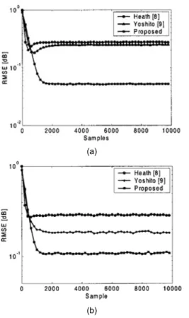
Fig. 3 shows the RMSE of the channel estimates from

existing algorithms and the proposed algorithm. From

these figures, we can see that the proposed algorithm

always performs better than others. By inspection, we

can observe that RMSE values of the proposed method

are decreased more or less 6-10 dB, and 1-2 dB under

20 dB, and 10 dB, respectively. Clearly, we can observe

the significant improvement of the proposed algorithm over existing algorithms.

(a)

(b)

그림 3. 제안 알고리즘과 기존 알고리즘의 RMSE 비교 (a) SNR=20dB and (b) SNR=10dB

Fig. 3 RMSE comparison of the proposed and existing

Ⅴ. Conclusion

In this paper, an approach to channel identification has been presented. The method is based on eigenvalue decomposition. The eigenvector corresponding to the minimum eigenvalue of the covariance matrix of the received signals contains the channel impulse response.

And we use a simple constrained LMS algorithm to estimate iteratively the eigenvector corresponding to the minimum eigenvalue. In comparison with algorithms, the proposed one seems to be more efficient in a low

SNR channel and much more accurate.

REFERENCES

[ 1 ] S. Haykin, Adaptive Filter Theory. Englewood Cliffs, NJ:

Prentice-Hall, 1996.

[ 2 ] L. A. Baccala and S. Roy, “A new blind time-domain channel identification method based on cyclostationarity,”

IEEE Signal Processing Letters, vol. 1, no. 6, pp. 89-92,

[ 3 ] L. Tong, G. Xu, and T. Kailath, “Blind identification and equalization based on second order statistics: A time domain approach,” IEEE Trans. Inform. Theory, vol. 40, no. 2, pp. 340-349, Mar. 1994.

[ 4 ] G. Xu, H. Liu, L. Tong, and T. Kailath, “A least-squares approach to blind channel identification,” IEEE Trans.

Signal Processing, vol. 43, no. 12, pp. 2982-2983, Dec.

1995.

[ 5 ] L. Tong and S. Perreau, “Multichannel blind identification:

from subspace to maximum likelihood methods,” Proc.

IEEE, vol. 86, no. 10. pp. 1951-1968, Oct. 1998.

[ 6 ] D. Gesbert and P. Duhamel, “Unbiased blind adaptive channel identification and equalization,” IEEE Trans.

Signal Processing, vol. 48, no. 1, Jan. 2000.

[ 7 ] O. L. Frost III, “A algorithm for linearly constrained adaptive arrays,” Proc. IEEE, vol. 60, no. 8, pp. 926-935, Aug. 1972.

[ 8 ] R. W. Heath Jr., S. D. Halford, and G. B. Giannakis,

“Adaptive blind channel identification of FIR channels for viterbi decoding,” in Proc. 31th Asilomar Conf. Signals,

Syst., and Comput., 1997.

[ 9 ] Y. Higa, H. Ochi, S. Kinjo, and H. Yamaguchi, “A gradient type algorithm for blind system identification and equalizer based on second order statistics,” IEICE Trans. Fundamentals, vol, E32-A, no. 8, pp. 1544-1551, Aug. 1999.

[10] T. J. Endres, S. D. Halford, C. R. Johnson, and G. B.

Giannakis, “Simulated comparisions of blind equalization algorithms for cold startup applications,” Int J. Adaptive

Contr. Signal Process., vol. 12, no. 3, pp. 283-301, May

[11] D. L. Goekel, A. O. Hero, and W. E. Stark, “Data-recursive algorithms for blind channel identification in oversampled communication systems,” IEEE Trans. Signal Processing, vol. 46, no. 8, pp. 2217-2220, Aug. 1998.

황지원(Jeewon Hwang)

1995년: 전북대학교 전자공학과 공학박사 2003년: 뉴질랜드 CPIT 방문교수

1992년 ~ 현재 전북대학교 IT정보공학과 교수

※관심분야 : 컴퓨터구조, Cognitive Radio, LTE 요소기술

조주필(Juphil Cho)

2001년 : 전북대학교 전자공학과 공학박사 2000년 ~ 2005년 : ETRI 이동통신 연구단 선임연구원 2006년~2007년 : ETRI 초빙연구원

2011년 : 미국 USF, 교환교수

2005년~ 현재 : 군산대학교 전파공학과 부교수

※관심분야 : Cognitive-Radio, 주파수 융합기술, LTE