IEG 환경지질연구정보센터

1. Introduction

The radar wave coherence produces “speckle” in SAR imagery. This phenomenon gives to the images a granular appearance that complicates image analysis and interpretation in remote sensing tasks.

Although it is a deterministic phenomenon due to the coherent processing of terrain backscattering signals, the speckle contribution is often considered as noise.

A major issue for the use of synthetic aperture radar

(SAR) imagery is to remove speckle without destroying important image features.

Speckle noise is supposed to be dependent on the signal intensity in the sense that the noise level increases with the brightness. Many approaches have been proposed to reduce the speckle effect in coherent imaging. Early works used the adaptive filters based on linear minimum mean square error by taking local statistics. The best-known filters include the Lee filter (Lee, 1986), Frost filter (Frost et al.,

Boundary-adaptive Despeckling : Simulation Study

Sang-Hoon Lee^†

Department of Industrial Engineering, KyungWon University, SeongNam, Korea

Abstract :In this study, an iterative maximum a posteriori (MAP) approach using a Bayesian model of Markovrandom field (MRF) was proposed for despeckling images that contains speckle. Image process is assumed to combine the random fields associated with the observed intensity process and the image texture process respectively. The objective measure for determining the optimal restoration of this “double compound stochastic” image process is based on Bayes’ theorem, and the MAP estimation employs the Point-Jacobian iteration to obtain the optimal solution. In the proposed algorithm, MRF is used to quantify the spatial interaction probabilistically, that is, to provide a type of prior information on the image texture and the neighbor window of any size is defined for contextual information on a local region. However, the window of a certain size would result in using wrong information for the estimation from adjacent regions with different characteristics at the pixels close to or on boundary. To overcome this problem, the new method is designed to use less information from more distant neighbors as the pixel is closer to boundary. It can reduce the possibility to involve the pixel values of adjacent region with different characteristics. The proximity to boundary is estimated using a non-uniformity measurement based on standard deviation of local region. The new scheme has been extensively evaluated using simulation data, and the experimental results show a considerable improvement in despeckling the images that contain speckle.

Key Words :

Received June 30, 2009; Revised June 30, 2009; Accepted July 1, 2009.

†Corresponding Author: Sang-Hoon Lee ([email protected])

1982), Kuan filter (Kuan et al., 1985). The Frost filter was designed as an adaptive Wiener filter that assumed an autoregressive exponential model for the scene reflectivity. Kuan considered a multiplicative speckle model and designed a linear filter based on the minimum mean-square error criterion, optimal when both the scene and the detected intensities are Gaussian distributed. The Lee filter was a particular case of the Kuan filter based on a linear approximation made for the multiplicative noise model. More recent works include the use of anisotropic diffusion. Diffusion algorithms remove noise by modifying the image via a partial differential equation. Since Perona and Malik (1990) introduced the formulation of anisotropic diffusion using an edge stopping function, the PDE-based approaches have been suggested to remove speckle noise with effective edge preserving. They include speckle- reducing anisotropic diffusion (SRAD) (Yu et al., 2002), detail-preserving anisotropic diffusion (DPAD) (Aja-Fern?ndez and L?pez, 2006) and oriented speckle reducing anisotropic diffusion (OSRAD) (Krissian et al., 2007). SRAD is the edge sensitive diffusion for specked images, in the same way that conventional anisotropic diffusion is the edge-sensitive diffusion for images corrupted with additive noise, and DPAD is a more robust way to estimate the coefficient of variation using different neighborhood sizes for filtering and noise estimation.

The OSRAD filter combines SRAD with a matrix anisotropic diffusion and add a non-scalar component to the SRAD filter that can perform directional filtering of the image the structures. In most cases, the corrected image is restored through a series of iteration.

Lee (2007a) suggested an iterative approach for despeckling the SAR images that are corrupted by multiplicative speckle noise. It is a maximum a posteriori (MAP) method using a Bayesian model

based on the lognormal distribution for image intensity and a Markov random field (MRF) for image texture. When the image intensity is logarithmically transformed, the speckle noise becomes approximately Gaussian additive noise and it tends to a normal probability much faster than the intensity distribution (Arsenault and April, 1976).

The MRF is incorporated into digital image analysis by viewing pixel type s as states of molecules in a lattice-like physical system defined on a Gibbs random field (GRF) (Georgii, 1979). Because of the MRF-GRF equivalence resulted from the Hammersley-Clifford theorem (Kindermann and Snell, 1982), the assignment of an energy function to the physical system determines its Gibbs measure, which is used to model molecular interactions. Thus, this assignment also determines the MRF. The MAP estimation of noise-free imagery employs a Point- Jacobian iteration (Varga, 1962). The Point-Jacobian iteration MAP (PJIMAP) scheme was proved to yield much better results than the conventional approaches for the speckle reduction (Lee, 2007a). Lee (2007b) also proposed an alternative adaptive scheme for the MAP estimation of Point-Jacobian iteration (AIMAP). In the adaptive approach, the parameters are computed using the updated data at each iteration, while the PJIMAP uses the parameters estimated with the original observation. AIMAP gives an improvement in speckle reduction by using the adaptive parameters for the Ponit-Jacobian iteration.

However, AIMAP is sensitive to the size of the

window employed to define the neighborhood system

of MRF. Using a large window of high order

neighborhood system is suitable for homogeneous

inner area, but results in smoothing over the boundary

between different regions and possibly fading the

detailed features. In this study, an approach to employ

variable sizes of the neighbor window depending on

the location has been proposed. According to how

near to boundary, the new scheme assigns different values into the parameters related to smoothing. The proximity to boundary is measured by a simple statistics based on local standard deviation.

The purpose of this paper is to develop and design a boundary-adaptive scheme of despeckling images that contain speckle through an extensive simulation study. The paper is organized as follows. Section 2 contains a brief description of the Point-Jacobian iteration approache, which was proposed for speckle removal in the previous works. In Section 3, the boundary-adaptive scheme proposed in this study is presented in detail. The experimental results of simulation data are reported to choose appropriate input constants required for the new scheme in Section 4. Finally, the conclusions are stated in Section 5.

2. Point-Jacobian Iteration for MAP Estimation

Image processes are assumed to combine the random fields associated with intensity and texture respectively. Given a noisy image from this double compound stochastic image process, the objective measure of determining the optimal restoration can be established using Bayes’ theorem. The Bayesian model utilizes the parameters related to smoothing and bonding strength between neighbors. The smoothing parameter represents the relative strength of prior belief of spatial smoothness compared to observational information, and the bonding strength is represented by nonnegative coefficients associated with local texture model.

Given an observed image Y, the Bayesian MAP estimation is to find the mode of the posterior probability distribution of the noise-free vector X, or equivalently, to maximize the log-likelihood function

lPN = ln P(YΩX) + ln P(X). (1) The MRF is used to quantify the spatial interaction probabilistically, that is, to provide a type of prior information on the image texture. Due to the MRF- GRF equivalence (Kindermann and Snell, 1982), an MRF is determined with a Gibbs measure. Let I

= {1,2,…,n} be the index set of the pixels in the image.

If R

is the index set of the neighbor pixels of the ith pixel, R = {R

| i ∈ I

} is the neighborhood system of I

. A “clique” of {I

, R}, c, is a subset of I

such that every pair of distinct indices in c represents pixels which are mutual neighbors, and C denotes the set of all cliques. A GRF relative to the graph {I

, R} on X is defined as

P(X) = Z

exp{

E(X)

(2) E(X) = V

(X) (energy function)

where Z is a normalizing constant and V

is a potential function which has the property that it depends only on X and c. Specification of C and V

is sufficient to formulate a Gibbs measure for the local texture model. A particular class of GRF, in which the energy function is expressed in terms of non- symmetric “pair-potentials,” is used in this study (Kindermann and Snell, 1982). Here, the energy function of GRF is specified as a quadratic function of X = {x

, i∈I

} which defines the probability structure of the texture process:

E

(X) = a

(x

x

)

(3) where C

is the pair-clique system and a

is a nonnegative coefficient which represents the

“bonding strength” of the ith and the jth pixels.

Using the intensity model of Gaussian additive noise and the texture model of GRF, the log- likelihood function of Eq. (1) is:

lPN ∝

(Y

X)¢S S

(Y

X)

X¢BX (4) where S S is the covariance matrix of X and B = {b

} is

(i,j)∈C

S

i∈I

S

c∈C

S

the bonding strength matrix where

_

a

for (i,j) ∈C

b

= a

for (i = j) .

0 otherwise

Since the log-likelihood function of Eq. (4) is convex, the MAP estimate of X is obtained by taking the first derivative:

S

S

(Y

X)

(5) By solving Eq. (5) with the Point-Jacobian iteration (Varga, 1962), the noise-free intensity can be recovered iteratively (Lee, 2007a) from the observation Y = {y

| i∈I

}: at the kth iteration for ∀i

∈I

, given an initial estimate, ˆ x

= y

,

x ˆ

= ( ^s

^y

^b

^{x ˆ}

) ^{. (6)}

The iteration converges to a unique solution since g(M

)<1 where g( )denotes the spectral radius (Cullen, 1972) and

Md

= diagonal{s

_2

+ b

, i∈I

} .

= {b

= b

Ω b

= 0}

3. Boundary-Adaptive Parameter Estimation

Various regions constituting an image can be characterized by textural components. The bonding strength coefficients of Eq. (3) are associated with local interaction between neighboring pixels and can provide some contextual information on the local region.

1) Bonding Strength Coefficient

For the (k+1)th iteration, given the estimate of the previous iteration, Xˆ

= { ˆx

, i∈I

}, the posterior probability of X can be stated under the assumption of x ˆ

~ N(x

, s

):

f(XΩˆ X

) ∝

( ˆ X

X)¢S S

( ˆ X

X)

X¢BX, (7) where S S

= diagonal{s

, i∈I

}. The Bayesian MAP estimation of X can be then considered as an optimization problem:

{ ^a

^{( x}

^x

⁾

} ⁽⁸⁾

subject to s

(ˆ x

x

)

≤r,∀i∈I

where r is a given constant related to the distribution of ˆ x

. Since the objective function and the constraints are convex, the optimization of Eq. (8) is restated using a Lagrange multiplier as:

{ [ ^a

^{( x}

^x

⁾

^+l

^{( s}

^{(ˆ x}

^x

⁾

^{r )} ]} ^.(9)

or equivalently, if j

= 1/l

and q

= a

j

,

{ ^j

[ ^q

^{( x}

^x

⁾

^{+ ( s}

^{(ˆ x}

^x

⁾

^{r )} ]} ^.(10)

Suppose {q

, j ∈I

Ω q

= 1} as the weights associated with the relative strength of interaction between the individual types of pair-cliques at the ith pixel. These interaction coefficients represent a textural component for the local region corresponding to the ith pixel, and, adopting a Bayesian interpretation, j

is referred to as a parameter that represents the relative strength of prior beliefs compared to information on the observation.

From Eq. (10), if the normalized interaction coefficients are predetermined, {j

} are then estimated by solving the first derivative equation system (Lee, 2007b):

j

= (11)

It is natural that neighboring pixels with more similar values have a higher probability of having the same intensity level and the bonding strength between pixels is inversely proportional to the distance between them. Under this supposition, the

j∈I

S

(i,j)∈C

S

i∈I

S

arg min

X

(i,j)∈C

S

i∈I

S

arg min

X

(i,j)∈C

S

i∈I

S

arg min

X

(i,j)∈C

S

1 s

+ b

(i,j)∈C

S

Ï Ô Ô Ô Ô Ó

r

s

S q

( x ^ˆ

x ˆ

)

(i,j)∈Cp

weight can be chosen:

q ˆ

= for (i, j)∈C

(12)

0 otherwise

where d

is the geometric distance between the ith and jth pixels, and the sample variance of local region can be used as an estimate of s

:

s ˆ

= (13)

where W

is the index set of the pixels belonging to the window that is centered at the ith pixel and associated with the neighborhood system of C

, n

is the number of the pixels of W

and x _

ik

is the average of {ˆ x

, i∈W

}.

If one of the neighbor pixels has a very close value with the center pixel value compared to them of the other neighbor pixels, the weight of this neighbor pixel is very large relatively, and the contextual information of neighborhood is then dominated by this pixel, even if other neighbors have right information. This problem can be alleviated by giving a limitation on the quadratic distance of pixel-pair in Eq. (12):

q ˆ

= for (i, j)∈C

(14)

0 otherwise

where

d

= max { ^{( x ˆ}

^{x ˆ}

⁾

^{, h}

^sˆ

} ⁽¹⁵⁾

and h

is a predetermined constant. The choice of smaller h

results in giving more weight to the neighbor pixels whose values are closer to the center pixel value. In Eq. (6), b

=

jˆ

qˆ

for i≠j and b

= jˆ

, and at the (k+1)th iteration of APJI,

x ˆ

= ( ^y

^{+ v}

^qˆ

^{x ˆ}

) ⁽¹⁶⁾

where v

= sˆ

jˆ

.

2) Boundary-Adaptive Parameter

The MAP estimation using the neighbor window associated with the pair clique system would use wrong information from adjacent regions for the pixels located in the region close to or on boundary.

To overcome this problem, the new method is designed to use a smaller size of the neighbor window and a lower value of the bonding coefficients as the location of pixels is closer to boundary. The small window can reduce the possibility to involve the pixel values of adjacent region with different characteristics, and the low value of the bonding coefficients can make the estimation fit to the own value of the pixel more than the values of the neighbor pixels.

Homogeneity is mainly related to the local information of an image and reflects how uniform an image region is. Since a region including boundary is non-uniform, the homogeneity plays important role to find the region close to or on boundary. As a proximity measure to boundary, this study uses a simple non-parametric statistics based on the sample standard deviation that describes homogeneity within local region. The proximity coefficient is defined in [0 1]:

p

= (17)

s

= ,

W

is the index set of the pixels belonging to the window centered at the ith pixel, n

the number of W

the pixels of and _

y

the average of observed values in W

. It is supposed that the measure of Eq. (17) has a

s

min

{s

} max

{s

}

min

{s

}

(i,j)∈C

S

1 1 + v

S

( x ^ˆ

_ x

)

n

d

_1

( x ^ˆ

x ˆ

)

d

( x ^ˆ

x ˆ

)

(i,m)∈C

S

Ï Ô Ô Ô Ô Ó

d

d

_2

d

d

_2 (i,m)∈C

S

Ï Ô Ô Ô Ô Ó

S

(y

_

y

)

n

larger value for the pixels closer to boundary. The boundary-adaptive bonding strength coefficients are estimated:

j

= (18)

q ˆ

= for (i, j)∈C

(19)

0 otherwise

d

= max { ^{( x ˆ}

^{x ˆ}

⁾

^{, (1}

^p

^)h

^sˆ

} ⁽²⁰⁾

where t is a constant associated with rapidity in reduction of window size. The proposed scheme is designed to use a smaller neighbor window, smaller constants of r in Eq. (11) and h

of Eq. (15) as the pixel considered is closer to the boundary. For larger t, the window size decreases more rapidly.

4. Experiments

A simple statistical model of multiplicative noise (Dainty, 1984) has been often used for the speckle reduction. A simple model of SAR imagery is usually given by

z

v

h

, i∈I

(20) where {h

} are multiplicative noise following a log- normal distribution. In this study, the adaptive Point- Jacobian iteration (APJI) was applied to the log- transformed intensity observation. First, the proposed scheme was extensively examined using simulation SAR data generated by the Monte Carlo method to evaluate the effect of the predetermined constants used in the algorithm.

For the Point-Jacobian iteration of Eq. (6), s

of Eq. (17) was used as the estimate of s

and the condition of convergence was defined as

≤k

(21)

where k

<< 1 is a given constant. The APJI scheme commonly requires three predetermined constants, the order of W

, r of Eq. (8) and h

of Eq. (15), and the boundary adaption requires two more constants, the order of W

in Eq. (17) and t of Eq. (19). In the boundary adaptive scheme, the local range for the estimation of proximity proximity to boundary should be larger than or equal to the neighbor area associated with C

. It is proper that W

, which defines local region to compute the proximity measure and the estimate of s

of Eq. (17), is chosen to have the same order as W

with a minimum order. In this study, the square windows that have the size of (2m+1)×

(2m+1) for the mth order were employed for W

and W

, k

was given with 0.01, and the minimum order of W

was set to the third.

If the number of scattering points per resolution cell is large in SAR, a fully developed speckle pattern can be modeled as the magnitude of a complex Gaussian field with independent and identically distributed real and imaginary components (Goodman, 1976). It leads to the Rayleigh distribution as the intensity distribution model. For the experiment, 16-bit simulation SAR images with the Rayleigh distribution were generated using 6 patterns.

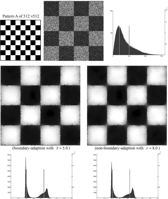
First, APJI was applied to the data simulated from Pattern A, a check-board pattern of 512×512. Fig. 1 shows in the first row the pattern, the simulated speckled-image and the histogram of observation data distribution. In the check-board pattern, the size of each square is 64 ×64, and it has 2 classes with the noise-free intensities of 200 and 500 respectively.

The bar in the histogram indicates noise-free intensity. The second row illustrates the despeckled images resulted from both of the APJI filters with and without boundary adaption. The figure includes the

S

s

n

S

Ωˆx

x ˆ

Ω n

p

r s ˆ

S q ˆ

( x ^ˆ

x ˆ

)

(i,j)∈Cp

d

d

d

d

_2 (i,m)∈C

S

Ï Ô

Ô Ô

Ô Ó

histograms that represent the distribution of the despeckled data in the third row. Tables 1 and 2 contain quantitative comparison between the algorithms with and without boundary adaption. For quantitative comparison, this study uses three

measures: Diff

, Error

and Error

. Diff

represents the level of difference between different regions on boundary defined as:

Diff

= max S ( ^{x ˆx}

^ˆx x

^{, 0} ) ⁽²²⁾

(i,j)∈Bn

Fig. 1. Despeckled sub-images (2nd row) and histogram of despeckled data (3rd row) resulted from APJI using Orderp= 9 and hd= 0.5 : In the 1st row, image pattern for simulation, simulated observation of sub-area and histogram of observed data (from left).

where B

is the index set of adjacent pair-pixels on boundary, x

and ˆx

the noise-free and despeckled intensities of the ith pixel respectively. The bigger Diff

is, the better the despeckled image is in contrast. Error

and Error

represents classification error in percent of two simple methods using the points of histogram valley as thresholds and the Euclidian distance from class mean-intensity respectively. The class mean-intensity is computed by averaging the despeckled intensities of the pixels belonging to each class. As the despeckled images agrees more with true pattern, the classification has smaller error. The histogram of despeckled data in Fig. 1 illustrates the histogram valley, which is pointed by arrow, and the class mean-intensity, whose value is corresponding to the x-coordinate of the bar. In the figures and tables, Order

represents the order of W

.

The first histogram of Fig. 1 implies that the simulated data are well distributed with a left-skew distribution as simulation of SAR observation. From the results of Tables 1 and 2, the boundary contrast is dependent on the values of three predetermined constants, h

, t and r. The large r is required for inner homogeneous area to relax higher speckle noise, but it may fail in preserving the edges between different regions. The value of r can be fixed at the stage of the system installment for the boundary-adaptive algorithm, which is designed to use a large value of r in inner area by multiplying the inverse of the proximity coefficient. An appropriate choice of r is a unit value (r = 1) since the sample variance of local region is used as the estimate of s

of Eq. (8). The resultant images in the second row of Fig. 1 show that the boundary-adaptive scheme less faded boundary especially at the corner, as well as relaxing speckle in inner area as much as the non-boundary-adaption does with a large r. The histograms in the third row indicate the results of both APJI schemes quite well

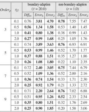
adaptive and non-boundary-adaptive APJIs applied to simulation data of Pattern A in Fig. 1

Orderpboundary-adaptionnon-boundary-adaption (= 20.0)(r = 1.0)

Diffb+ ErrorhErrord Diffb+ ErrorhErrord

0.1 0.76 3.81 4.70 0.78 7.55 7.47 3 0.5 0.56 1.34 1.58 0.53 1.40 1.45 1.0 0.41 0.80 1.38 0.38 0.99 1.43 2.0 0.27 0.99 1.68 0.25 1.05 1.76 0.1 0.74 3.89 3.63 0.76 6.93 6.91 5 0.5 0.53 0.99 1.46 0.52 1.70 1.77 1.0 0.37 0.88 1.51 0.35 1.27 1.86 2.0 0.26 1.08 1.80 0.22 1.10 2.35 0.1 0.72 2.40 3.05 0.75 7.44 6.79 7 0.5 0.52 1.09 1.36 0.52 2.00 2.16 1.0 0.36 0.74 1.54 0.33 1.71 2.30 2.0 0.25 0.92 1.79 0.21 1.33 2.72 0.1 0.71 2.20 2.64 0.76 7.02 6.88 9 0.5 0.51 0.95 1.26 0.52 2.33 2.54 1.0 0.35 0.80 1.51 0.32 1.76 2.69 2.0 0.25 0.90 1.85 0.20 1.58 3.06 boundary-adaption non-boundary-adaption

Order_p hd (t = 20.0) (r = 1.0)

Diff_b+ Error_h Error_d Diff_b+ Error_h Error_d

Table 2. Comparison of despeckled results of boundary- adaptive and non-boundary adaptive APJIs applied to simulation data of Pattern A in Fig. 1

boundary-adaption non-boundary-adaption (= 5.0)(r = 8.0)

?Diff?_(b+)?Error?_h?Error?_d?Diff?_(b+)?Error?_h?Error?_d 0.1 0.66 2.39 3.55 0.59 1.80 3.26 3 0.5 0.49 1.03 1.16 0.41 0.84 1.11 1.0 0.36 0.76 1.15 0.25 0.79 1.60 2.0 0.20 0.73 1.99 0.16 0.96 2.37 0.1 0.63 2.65 3.00 0.58 2.14 2.90 5 0.5 0.46 1.25 1.36 0.38 1.04 1.30 1.0 0.30 0.95 1.54 0.21 1.11 2.26 2.0 0.15 0.88 2.91 0.12 0.86 3.28 0.1 0.62 3.21 3.30 0.58 2.75 3.12 7 0.5 0.45 1.50 1.65 0.37 1.46 1.60 1.0 0.26 0.93 1.99 0.18 0.92 2.89 2.0 0.13 1.01 3.69 0.11 0.98 3.88 0.1 0.63 3.61 3.85 0.59 3.27 3.57 9 0.5 0.45 1.85 1.94 0.36 1.74 1.94 1.0 0.24 1.23 2.58 0.17 1.23 3.52 2.0 0.12 1.19 3.86 0.12 1.20 4.13 boundary-adaption non-boundary-adaption

Orderp h_d (t = 5.0) (r = 8.0)

Diffb+ Errorh Errord Diffb+ Errorh Errord

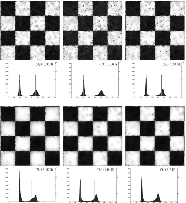
agree with the true pattern of two classes. Fig. 2 shows the effects of three input constants for the boundary-adaptive APJI filter on the despeckled results. As shown in Table 1, the despeckled images of the boundary-adaptive filter yielded smaller classification error compared to them of the non-

boundary-adaption when the boundary contrast of two results is similar. Table 2 shows that, when their classification errors are much of a muchness, the boundary-adaptive scheme has better boundary- contrast.

Next, the proposed boundary-adaptive APJI filter

Fig. 2. Despeckled sub-images and histogram of despeckled data resulted from applying Boundary-adaptive APJI with different sets of three constants of (Orderp, hd, t) to simulation data of Pattern A in Fig.1.

(3,0.5,10.0)

(9,0.5,10.0)

(5,0.1,10.0)

(5,1.0,10.0) (5,0.5,5.0)

(5,0.5,20.0)

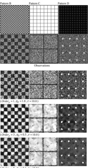
was applied to the simulation data generated from three patterns of 512 ×512 having more complicate structure. Fig. 3 displays the patterns used for simulation and the simulated data having speckle noise of Raleigh distribution in the first two rows, and the despeckled sub-images resulted from applying the boundary-adaptive APJI filter with different sets of three constants to the simulation data. Pattern B is a check-board pattern in which the size of each square is 16 ×16, Patterns C and D have thin lines and small

squares respectively. Tables 3, 4 and 5 contain the results that evaluate the despeckling of the APJI filters for the simulation data of Fig. 3. Except using the neighborhood system of order 1, the boundary- adaptive scheme demonstrated much better capability of despeckling the noisy data to agree with true pattern for complicate scene. For the neighborhood

Fig. 3. Despeckled sub-images resulted from applying Boundary-adaptive APJI with different sets of three constants to simulation data of Patterns B, C and D of 512×512 (1st and 2nd row).

Table 3. Comparison of despeckled results of boundary- adaptive and non-boundary-adaptive APJIs applied to simulation data of Pattern B in Fig. 3

boundary-adaption

(= 10.0)non-boundary-adaption(r = 2.0)

?Diff?_(b+)?Error?_h?Error?_d?Diff?_(b+)?Error?_h?Error?_d 0.1 1.00 26.66 16.02 1.00 21.04 15.94 1 0.5 0.84 14.84 12.68 0.80 15.05 12.35 1.0 0.73 10.14 10.22 0.67 8.78 9.94 0.1 0.76 7.32 7.61 0.78 9.70 9.46 3 0.5 0.56 4.28 4.45 0.54 4.94 5.08 1.0 0.40 3.79 4.54 0.36 6.44 5.30 0.1 0.77 9.65 8.68 0.81 11.43 10.66 5 0.5 0.56 5.06 5.02 0.54 5.79 5.81 1.0 0.39 6.54 6.11 0.32 5.23 5.31 0.1 0.83 11.99 11.01 0.87 12.86 12.10 7 0.5 0.56 13.31 11.51 0.55 6.65 6.50 1.0 0.43 32.21 15.02 0.32 36.15 7.72 boundary-adaption non-boundary-adaption

Order_p hd (t = 10.0) (r = 2.0)

Diff_b+ Error_h Error_d Diff_b+ Error_h Error_d

Table 4. Comparison of despeckled results of boundary- adaptive and non-boundary-adaptive APJIs applied to simulation data of Pattern C in Fig. 3

boundary-adaption(= 10.0)non-boundary-adaption (r = 2.0)?Diff?_(b+)?Error?_h?Error?_d?Diff?_(b+)?Error?_h

?Error?_d

0.1 1.00 11.13 24.93 0.99 9.53 24.94 1 0.5 0.86 6.83 21.17 0.80 6.20 20.72 1.0 0.75 5.14 17.01 0.68 4.80 16.57 0.1 0.72 6.54 8.14 0.73 10.29 13.19 3 0.5 0.50 3.17 3.84 0.34 5.39 6.19 1.0 0.34 5.23 6.43 0.20 6.87 9.82 0.1 0.71 5.52 6.38 0.74 10.95 11.68 5 0.5 0.49 4.85 5.87 0.23 7.92 12.90 1.0 0.31 6.28 9.75 0.14 8.75 15.81 0.1 0.72 5.76 5.74 0.79 10.87 10.84 7 0.5 0.52 5.72 7.42 0.18 9.48 17.36 1.0 0.35 7.04 11.93 0.13 10.41 19.52 boundary-adaption non-boundary-adaption

Orderp hd (t = 10.0) (r = 2.0)

Diffb+ Errorh Errord Diffb+ Errorh Errord

system of the lowest order, both algorithms of the APJI filter would produce the results to some extent fit to the observation rather than consistent with true pattern, and they then appear similarly. The use of the lowest order system may be better in visual interpretation for the scene of very complex structure, but is not suitable for further post-processing such as image classification. The results of the three tables

suggest for the data from a complicate scene that the ARJI filter uses relatively small Order

, but greater than one, is chosen for APJI filter is choose large h

for large Order

. It is also implied in the following experimental results of Table 6.

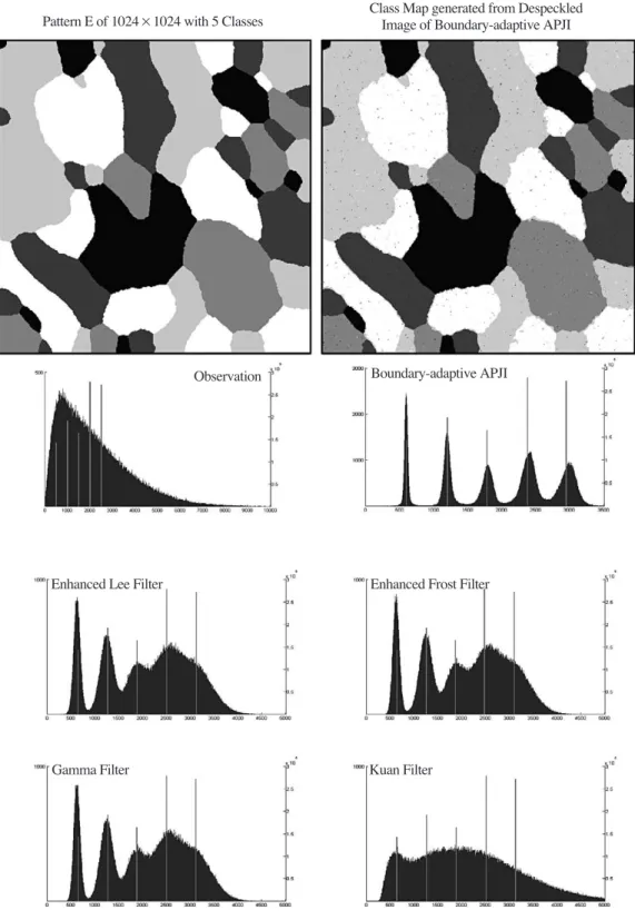
The boundary-adaptive scheme was tested using the data simulated from two patterns, shown in Figs.

4 and 5. The results were compared to them of the four adaptive filters, enhanced Lee filter, enhanced Frost filter, Gamma filter and Kuan filter, which are installed in ENVI 4.2. The experiment used the filter size of 5×5 for all the conventional methods. The histograms of the despeckled data exhibit superior performance of the APJI filter in these figures, and they include the class maps generated from the despeckled data by the simple histogram valley approach. As shown in the figures, all the conventional filters failed in producing the despeckled images to agree with the true pattern of 5 classes as much as the APJI filter did, and yielded very similar results except the Kuan filter. Tables 6 and 7 contains the evaluation measures of the results of the boundary-adaptive APJI filter with different predetermined constants and the conventional filters

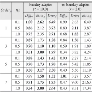
adaptive and non-boundary- adaptive APJIs applied to simulation data of Pattern D in Fig. 3

boundary-adaption(= 10.0)non-boundary-adaption(r = 2.0)

?Diff?_(b+)?Error?_h?Error?_d?Diff?_(b+)?Error?_h

?Error?_d

0.1 1.00 2.62 6.49 0.99 2.63 6.49 1 0.5 0.86 2.12 3.73 0.80 2.11 3.87 1.0 0.75 2.35 2.71 0.68 1.82 2.87 0.1 0.87 1.73 1.28 0.84 1.56 1.43 3 0.5 0.70 1.10 1.10 0.59 1.91 1.89 1.0 0.51 3.00 1.79 0.34 3.82 4.24 0.1 0.88 1.43 1.42 0.90 2.27 2.14 5 0.5 0.70 1.73 1.70 0.44 5.42 11.85 1.0 0.50 3.17 2.30 0.40 5.56 11.19 0.1 0.89 1.58 1.52 1.01 3.27 3.57 7 0.5 0.71 1.75 1.73 0.47 9.60 21.63 1.0 0.54 3.00 2.64 0.43 8.31 17.34 boundary-adaption non-boundary-adaption

Order_p hd (t = 10.0) (r = 2.0)

Diff_b+ Error_h Error_d Diff_b+ Error_h Error_d

Table 6. Evaluation of despeckled results yielded from boundary-adaptive APJIs using different sets of (Orderp, hd) with t = 10.0 for simulation data of Patterns E and F in Figs. 4 and 5

Orderp hd Pattern E hd Pattern F

Diffb+ Errorh Errord Diffb+ Errorh Errord

0.5 0.40 5.36 5.26 0.1 0.65 19.17 19.76

3 1.0 0.30 4.47 4.63 0.5 0.41 7.17 6.95

2.0 0.20 5.19 5.06 1.0 0.31 7.57 7.37

0.5 0.36 3.10 3.22 0.1 0.58 11.43 11.57

5 1.0 0.25 3.48 3.59 0.5 0.38 6.56 6.11

2.0 0.17 4.43 4.46 1.0 0.27 8.33 7.75

0.5 0.35 3.47 3.15 0.1 0.55 8.56 8.72

7 1.0 0.23 3.82 3.90 0.5 0.36 6.98 6.69

2.0 0.15 5.03 5.12 1.0 0.25 10.10 9.20

0.5 0.34 3.19 3.37 0.1 0.54 8.36 7.93

9 1.0 0.22 4.35 4.43 0.5 0.35 8.09 7.63

2.0 0.15 5.94 5.91 1.0 0.24 11.43 11.05

Orderp hd Pattern E hd Pattern F

Diffb+ Errorh Errord Diffb+ Errorh Errord

Fig. 4. Histograms of despeckled data resulted from applying Boundary-adaptive APJI with (Orderp= 5, hd= 0.5, t = 10.0), and four conventional adaptive filters using filter size of 5×5 to simulation data of Pattern E.

Observation

Enhanced Lee Filter

Gamma Filter Kuan Filter

Enhanced Frost Filter Boundary-adaptive APJI

Pattern E of 1024×1024 with 5 Classes Class Map generated from Despeckled Image of Boundary-adaptive APJI

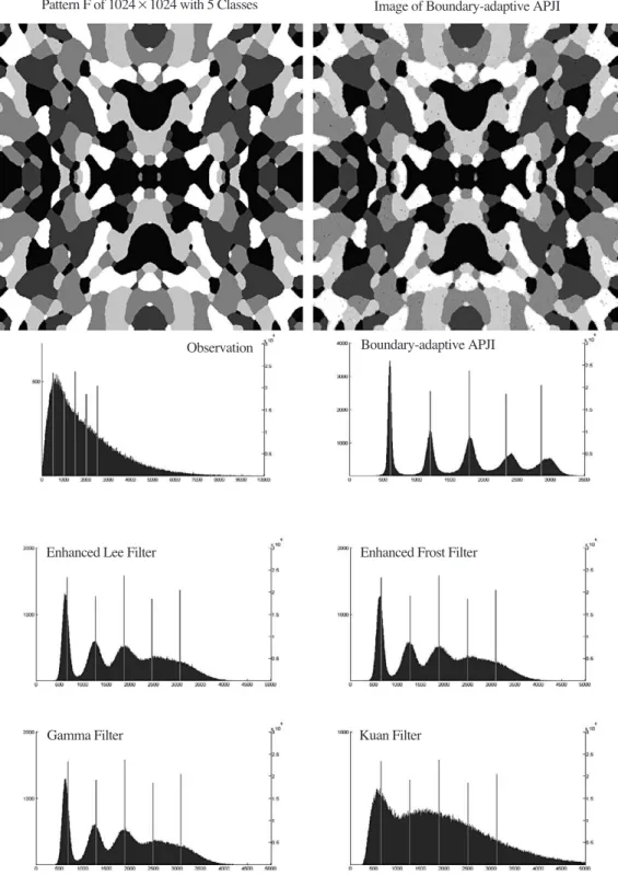
Fig. 5. Histograms of despeckled data resulted from applying Boundary-adaptive APJI with (Orderp= 5, hd= 0.5, t = 10.0), and four conventional adaptive filters using filter size of 5×5 to simulation data of Pattern F.

Observation

Enhanced Lee Filter

Gamma Filter Kuan Filter

Enhanced Frost Filter Boundary-adaptive APJI Pattern F of 1024×1024 with 5 Classes

Class Map generated from Despeckled Image of Boundary-adaptive APJI

respectively. The evaluation of the results of Pattern F in Table 6 indicates that it is a good choice to use smaller h

for larger Order

and, conversely, larger h

for smaller Order

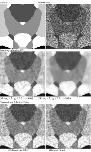
. As shown in Table 7, the performance of the conventional filters suffers by comparison with the proposed filter. Note that the Error

value of original simulation data of Pattern E

is 20.4%. Fig 6. shows the pattern and observation of sub-area including the despeckled sub-images resulted from the boundary-adaptive APJI filters and the conventional adaptive filters.

5. Conclusions

In this study, a boundary adaptive iterative scheme for despeckling images that contain speckle was developed by evolving the Point-Jacobian iteration MAP filter proposed in Lee (2007a). The use of large window results in improper smoothing in the boundary area of small regions. A larger window smoothes the image to some extent and results in fading the detailed features existed in the scene. This problem can be overcome by using the boundary- adaptive scheme to employ the neighbor windows of variable size according to how near to boundary. The proximity to boundary is estimated by the non- uniformity measurement.

This study extensively experimented using simulation data to properly choose the predetermined constants, Order

, h

and t for the boundary-adaptive algorithm. The proposed scheme yields better results with the neighborhood system of higher order for the image of plain structure, while using the lower order for the image of complicate structure. It is suggested to choose Order

in the range of 3 and 7. For larger Order

, smaller h

works better, and, conversely, larger h

for smaller Order

. The best choice of h

would be between 0.5 and 1.0. Though the experimental results related to the choice of t are not presented in this paper, it is suggested to choose between 5.0 and 20.0, and the lager t, the more boundary-contrast, as shown in Tables 1 and 2.

Table 7. Comparison of despeckled results of three conventional adaptive filters using filter size of 5×5 applied to simulation data of Patterns E and F in Figs. 4 and 5 Filter Pattern EPattern F

Diffb+ ErrorhErrord Diffb+ ErrorhErrord

Enhanced Lee 0.38 18.28 15.15 0.40 17.89 14.60 Enhanced Frost 0.26 18.36 14.84 0.28 18.04 14.82 Gamma 0.24 19.11 14.68 0.26 16.89 14.95

Filter Pattern E Pattern F

Diffb+ ErrorhErrord Diffb+ ErrorhErrord

Fig. 6. Despeckled sub-images resulted from applying Boundary-adaptive APJI and two conventional adaptive filters to simulation data of Pattern F

Acknowledgements

This research was supported by the Kyungwon University Research Fund in 2009.

References

Aja-Fernandez, S. and C. Alberaola-Lopez, 2006. On the estimation of the coefficient of variation for anisotropic diffusion speckling filtering, IEEE Trans. on Image Proc., 15(9): 2694 - 2701.

Arsenault H. H. and G. April, 1976. Properties of speckle integrated with a finite aperture and logarithmically transformed, J. Opt. Soc.

Amer., 66: 1160-1163.

Cullen, C. G., 1972. Matrices and Linear Transformations. Reading, MA: Addison- Wesley.

Dainty, J. C., 1984. Laser Speckle and Related Phenomena, Second Enlarged Edition.

Frost, V. S., J. A. Stiles, K. S. Shanmugan, and J. C.

Holtzman, 1982. A model for radar images and its application to adaptive digital filtering of multiplicative noise, IEEE Trans. Pattern Anal. Mach. Intell., 4: 157-165

Georgii, H. O., 1979. Canonical Gibbs Measure.

Berlin, Germany: Springer-Verlag.

Goodman, J. W., 1976. Some fundamental properties of speckle, J. Opt. Soc. Amer., 66: 1145-1150.

Kindermann R. and J. L. Snell, 1982. Markov Random Fields and Their Application, Providence, R. I.: Amer. Math. Soc.

Krissan. K., C-F. Westin, R. Kikinis, and K.

Vosburgh, 2007. Orientee speckle reducing anisotropic diffusion, IEEE Trans. on Image Proc., 16(5): 1412-1424.

Kuan, D. T., A. A. Sawchuk, and P. Chavel, 1985.

Adaptive noise smoothing filter for images with signal-dependent noise, IEEE Trans.

Pattern Anal. Machine Intell., 7: 165-177.

Lee, J. S., 1986. Speckle suppression and analysis for synthetic aperture radar, Opt. Eng., 25: 656- 643.

Lee, S-H, 2007a. Speckle Removal of SAR Imagery Using a Point-Jacobian Iteration MAP Estimation, Korean J. Remote Sens., 23(1):

33-42.

Lee, S-H, 2007b. Adaptive Iterative Despeckling of SAR Imagery, Korean J. Remote Sens., 23(5): 455-464.

Perona, P. and J. Malik, 1990. Scale space and edge detection using anisotropic diffusion, IEEE Trans. Pattern Anal. Machine Intell., 12: 629- 639.

Varga, R. S., 1962. Matrix Iterative Analysis, Englewood Cliffs, NJ: Prentice-Hall.

Yu, Y., and S. Acton, 2002. Speckle reduction

anisotropic diffusion, IEEE Trans. on Image

Proc., 11(11): 1260-1270.