Modelling of Wind Wave Pressure and Free-surface Elevation using System Identification

Journal of Korean Society of Coastal and Ocean Engineers 25(6), pp. 422~432, Dec. 2013 http://dx.doi.org/10.9765/KSCOE.2013.25.6.422

422

Modelling of Wind Wave Pressure and Free-surface Elevation using System Identification

시스템 식별기법을 활용한 파압과 해수면 모델링

Witold Cie´slikiewicz* and Jordan Badur*

위톨드 키에스키윅즈*·요르단 바두르*

Abstract: A System Identification method to develop parametric models linking free surface elevation and wave pressure is presented and two models are built allowing for either wave pressure or free surface elevation simulation.

Linear, time invariant model structures with static nonlinearities are assumed and solutions are sought in a form of autoregressive model with extra input (ARX). An arbitrary chosen free-surface elevation and wave pressure dataset is used for estimation of the models, which are subsequently verified against datasets with similar pressure gauge depth but different free-surface elevation spectra due to different meteorological conditions. It is shown that free- surface simulation using System Identification methods can perform better than traditional linear transfer function derived from linear wave theory (LTF), while wave pressure simulation quality using presented methods is generally similar to that obtained with corrected LTF.

Keywords: system identification; wind waves, free surface elevation, sea wave pressure, autoregressive model, ARX model, linear transfer function, wind wave spectrum, free surface records, pressure records.

요 지 :해수면과 해저파압을 연계하는 모수 모형을 개발하기 위한 시스템 식별법을 제시하였다. 비선형 고정변수

를 포함한 선형 시불변 모형 구조를 가정하고 추가적인 입력자료를 갖는 자기회귀모형 (ARX)을 이용하여 해저파 압 시계열자료로부터 해수면 시계열자료를 또는 해수면 시계열자료로부터 해저파압 시계열자료를 추출하는 방법을 제시하였다. 임의로 선정된 해수면과 해저 파압 자료를 이용하여 모형을 검증하였으며, 유사한 해저수심의 파압자 료와 다른 해상 기상조건으로 생성된 해수면 스펙트럼 자료를 통해 재검증하였다. 시스템 식별법을 이용한 방법이 전통적인 선형파 이론을 이용한 선형전송함수(LTF) 방법보다 전반적으로 더 정확하게 수행됨을 확인하였다. 또한 본 논문에서 제시된 방법으로 추정된 해저 파압 시계열모의는 수정 선형전송함수 (corrected LTF)에 의한 결과와 유사 함을 확인하였다.

핵심용어 :시스템 식별법, 풍파, 해수면, 해저파압, 자기회기모형, ARX 모형, 선형전송함수, 풍파스펙트럼,

해수면 시계열자료, 파압 시계열자료

1. Introduction

Relations between wave pressure and free surface eleva- tions have been applied to field measurements since 1947, when Folsom (1986) and Seiwall (1947) used pressure gauge to measure free surface elevations. Since then, a number of methods to obtain free-surface elevations from wave pressures have appeared whereas almost no interest was shown in modelling wave pressures on the basis of free-surface elevation. This obviously results from the fact, that it is usually easier to measure wave pressure than sur- face elevation. However, in some cases, such as apparatus

failure, a possibility for obtaining wave pressures from the free-surface records might be useful. Also, in some mari- time engineering applications, measuring pressure is more difficult than recording free-surface elevations. For exam- ple, it is possible to collect in a relatively easy way accurate measurements of water surface elevations using remote sensing techniques with a down-looking laser device installed on an offshore platform. In such situations it is suf- ficient to install underwater measuring equipment for a lim- ited period of time only, allowing model construction and estimation of its parameters. Then, measured time series of free-surface elevations may be used to provide the wave

*그단스크 대학, 해양학과 교수(Corresponding author : Witold Cie´slikiewicz, University of Gransk, Institute of Oceanography, Al. Marszalka Pilsudskiego 46, 81-378 Gdynia, Poland, Tel.: +48-58-523-6875, Fax: +48-58-523-5531, [email protected])

pressure data via the model developed.

Most of the procedures transforming wave pressure series into surface elevations time series can be modified to apply them in the reverse direction. These methods can either work globally (processing entire series at a time) or locally (small part of a series is processed). Global methods include:

- Linear Transfer Function (LTF) as summarized by Bishop and Donelan (1987), Tsai and Young (2001), Grace (1970);

- Nonlinear modification to LTF developed by Hashim- oto et al. (1997) on the basis of Tick’s paper (1959);

- Empirical Transfer Functions presented by Kou and Chiu (1994). The following local methods have been recently developed:

- Local Sinusoid Approximations (LSA) and empirical LSA methods by Nielsen (1989);

- Local Polynomial Approximations method (LPA) developed by Fenton (1986) and simple LPA by Fenton and Christian (1989);

- Local Fourier Approximations (LFA) presented by Sobey (1992), Barker and Sobey (1996 and 1997).

Linear Transfer Function (LTF) method is a simple deri- vation from linear wave theory: Fourier transform of free- surface elevation is multiplied by transfer function L(f), then transformed back to time domain and finally scaled by gravity and water density ρg. L(f) takes the famil- iar form of

with the wave number k related to the frequency f via dis- persion relation, vertical coordination z and mean water depth h. This method is still the most frequently used one despite its inaccuracy shown by Hom-ma et al. (1966), Grace (1970), Cavaleri (1980), Bisel (1982), Lee and Wang (1984), Wang et al. (1986) as well as authors using local methods listed above.

The method is generally recognized as working well in laboratory tests for linear waves, especially when the pres- sure gauge is installed at relatively high z-elevation (Bisel, 1982; Bishop and Donelan, 1987; Tsai et al., 2005). For nonlinear waves, LTF method fails to model high and low frequency behavior of processed series. Partially this results from cutting theoretical transfer function at some fre- quency f_c by setting its values to 0 for frequencies f_c and higher. Otherwise the infinitely increasing LTF multiplied by the pressure spectra would produce false values in high frequency region of the simulated free-surface elevation

spectra. Therefore, the linear transfer function is truncated, which results in producing surface elevation series with no energy contained at frequencies f_c and higher (Lee and Wang, 1984). Moreover, LTF is commonly multiplied by an empirical constant whose value seems to depend on loca- tion. Review of values can be found in Grace (1970) as well as in Bishop and Donelan (1987). Further empirical LTF developments by Kuo and Chiu (1994) clearly oversim- plify the transfer function, replacing water depth and gauge depth dependency with a single empirical modification.

That resulted in overestimating wave heights by as far 30%

during a field experiment reported in (Tsai et al., 2005).

Linear Transfer Function method can be corrected in high frequency region as suggested by Hashimoto et al. (1997) by setting LTF values for frequencies higher than f_c equal to a constant value referring to f_c. Hashimoto et al. (1997) pro- posed a new method to determine f_c based upon analytical properties of expressions for weakly nonlinear, second order spectra given by Tick (1959).

Local methods start with fitting sine curve (LSA), com- plex polynomial (LPA) or Fourier series (LFA) to a portion of pressure series surrounding the time of interest. Conse- quently, nonlinear dynamical equations are solved to find potential function and free surface elevation. Details can be found in: Nielsen (1989), Fenton (1986), Fenton and Chris- tian (1989), Sobey (1992), as well as in Barker and Sobey (1996 and 1997). Detailed comparison made by Townsend and Fenton (1996) showed that LPA work generally better than global methods (LTF) with regular waves and in cases when pressure gauge was set at greater depths. However, in a case of random waves LPA performed similarly to LTF due to higher noise-to-signal ratio. As Townsend and Fen- ton (1996) used only water tank generated data, LPA per- formance in field conditions remains unknown. Since fitting a polynomial to a signal is sensible to high noise-to- signal ratio, the procedure might perform not so well in transforming elevations to pressures. This might result from fitting a complex polynomial to a more noisy free surface elevation series. LSA, in turn, was found by Townsend and Fenton (1996) more robust against the noise. However, a disadvantage of the LSA methods is the failure just above the trough of the wave (Townsend and Fenton, 1996).

In this study we apply System Identification (SI) tech- niques to develop models transforming free-surface eleva- tions into wave pressures. In general, SI is concerned with constructing dynamic models of a system in which vari- ables of different kinds interact and produce observable sig- ξˆ t( )

L f a h(; , )= cosh[k f( ) z h⋅( + )]⁄cosh[k f( ) h⋅ ]

nals that are called outputs and which are of interest to us.

The system is simulated by external signals that are called inputs. We say the system and its components are dynamic when the current output values depend not only on the cur- rent input but also on their earlier values.

In the presented paper we suggest that it is possible to create two linear time invariant dynamic models linking the free-surface elevation and wave pressure series: one allow- ing for wave pressure simulation using free-surface eleva- tion as an input variable and second for free-surface elevation simulation using wave pressure as input data.

Obviously, on shallow water such a SI model is valid only for a given location, mean water level and-the most important-for a constant distance between the mean water level and pressure transducer depth. Furthermore, a linear model estimated in time domain using narrow-banded data will be most reliable when applied to input data with most of the spectral energy located close to the spectral band of estimation data. As the spectral density distribution S(f) over the frequency f can be roughly characterized by the

mean energy wave period it

might be feasible to the combine spectral information with the pressure transducer depth z and the water depth using the value of linear transfer function L_E taken at , i.e.

. The use of a simple rescaling coefficient based upon L_E might increase the reliability of simulation in case when the spectral properties of input data differ from the properties of estimation data.

In consequence, presented SI models can be applied to replace data occasionally disturbed due to equipment fail- ure or conservation or to monitor data consistency in real time. Further research is being directed to extend the mod- els onto wider transducer depth range and provide better simulation in case of input with spectra located outside the original band of estimation data.

System Identification techniques have been successfully applied, among others, to model wave velocities and accel- erations based on free-surface records by Cieœlikiewicz and Gudmestad (2001 and 202) as well as to Morrison equation improvement by Stansby et al. (1992), Selvam et al. (2001). Moreover, nonlinear System Identification meth- ods are a typical tool in marine engineering applications such as ship dynamics (Bendat, 1997; Faltisen, 1990; Mulk, 1994) or structure modelling (Bhattachararyya et al., 2001).

This paper extends results presented in previous studies (Cieœlikiewicz and Gudmestad ,2001 and 2002) by applica- tion of SI methods to either free-surface elevation or wave

pressure simulation and rescaling model results to use in case of slightly different (within 1 m range) pressure gauge depth, water depth and different sea state as manifested by mean energy wave period T_E differing from 3.9 to 5.6 s and signifi- cant wave height from 0.9 to 1.7 m in Table 1.

2. System Identification Procedures

This section briefly presents the framework of traditional System Identification techniques, which will be used in var- ious applications: model structure and input/output data will be changed. In particular, the wave pressure simula- tion model will use transformed series of free-surface ele- vation as an input and free-surface elevation model will use transformed wave- pressure as an input.

Let Y(t) denotes the output data sequence of the system, i.e., pressure record p_t in case of wave pressure simulation.

The input data vectors Q_t of N_Q dimension are composed of the free-surface elevation sequence .We include the random disturbance as an additive filtered white noise. We assume in this study that the wave system can be described by a linear time-invariant model which is specified by the sequence of impulse response series g_q(k), q = 1, ..., N_Q and the weighting function h(k) of the random additive distur- bance, , and, possibly, the probability den- sity function of the white-noise εt. It is worth noting, that despite the assumption of a linear model we are still able to incorporate in a system the nonlinearities that have the character of a static nonlinearity at the input side, while the dynamics of the system itself is linear. In case the nonlin- earity is known, say as a function F, a certain input variable T_E ^=[∫f^–1S f( ) fd^]⁄[∫^{S f( ) fd]}

f_E=T_E^–1 L_E =L f(_E;z h, )

ζ t( )

k=0 1, , ,… ∞

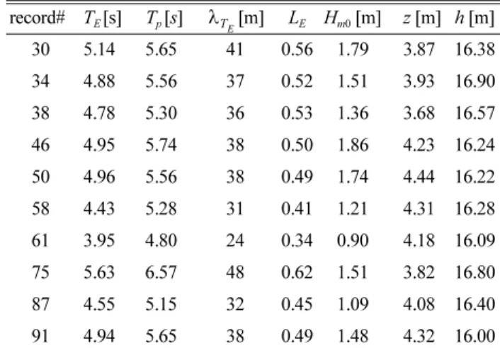
Table 1. Free-surface elevation record #, mean energy wave period TE, peak wave period Tp, wave length associated with TE, linear transfer function value LE, significant wave height Hm0, pressure transducer depth z and mean water depth h.

record# TE[s] Tp[s] [m] LE Hm0[m] z [m] h [m]

30 5.14 5.65 41 0.56 1.79 3.87 16.38 34 4.88 5.56 37 0.52 1.51 3.93 16.90 38 4.78 5.30 36 0.53 1.36 3.68 16.57 46 4.95 5.74 38 0.50 1.86 4.23 16.24 50 4.96 5.56 38 0.49 1.74 4.44 16.22 58 4.43 5.28 31 0.41 1.21 4.31 16.28 61 3.95 4.80 24 0.34 0.90 4.18 16.09 75 5.63 6.57 48 0.62 1.51 3.82 16.80 87 4.55 5.15 32 0.45 1.09 4.08 16.40 91 4.94 5.65 38 0.49 1.48 4.32 16.00

λ_TE

λ_TE

U(t) can be transformed into and the sys- tem can be treated as linear. We will have such a situation in this study. A complete model is given by the following rela- tionship (Ljung, 1987; S derstr m and Stoica, 1989):

(1)

in which f is the forward shift operator defined by f_Q(t) = Q(t + 1), G is the transfer function of the system and G(f)Q(t) is short for and for any

; (2)

Then

(3)

As mentioned above, we assume that the disturbance N can be described as filtered white-noise, so

(4)

where

(5)

Within SI we work with structures that permit the specifi- cation of G and H in terms of a finite number of numerical values. As is common, we assume that is Gaussian, in which case the PDF is specified by the first and second moments. Thus, a particular model (1) is entirely deter- mined in terms of a number of numerical coefficients which are included as parameters to be determined. The purpose of SI is to determine the values of those parameters. If we denote the parameters in question by the vector θ, and if we take into account the relation (4), the basic description of the modelled system becomes

(6) p_ε(·,θ), the PDF of ε(t); ε(t) white-nose

which is a set of models, each of them associated with a parameter value θ.

A commonly used way of parameterizing G_q and H is to rep- resent them as rational functions of f⁻¹and specify the numera- tor and denominator coefficient in some way (Ljung, 1987).

Such model structures, which are known as black-box models, were utilized in this study. A few different model structures were tested. In this paper the examples demonstrating the

results of SI with one of the simplest model structures, i.e., autoregressive with extra input (ARX) model structures for wave pressure will be presented. For the ARX model in multi- input single-output version equation (6) may be rewritten as

(7)

where is the autoregressive part while is the extra input of the ARX model in which

(8)

and for

(9)

The vectorial parameter θ to be determined is in this case composed of coefficients of the polynomials A and B_q

.. .

where are the orders of the multi-input single-output ARX model.

In the present study the models were estimated using least-squares methods. If we denote by N the length of the time series Y(t) and write

(11)

where , then the least-

squares estimate of the parameter vector is defined as

(12)

here arg[·] means “the minimizing argument of the func- tion.”

3. The experiment

The available data were collected on February 12 and March 10~11, 1976 at oceanographic tower Aqua Alta of CNR located in the northern Adriatic Sea approximately 7 Nm off the coast of Venice at 16 m water depth. Tower Q t( ) F U t= { ( )}

o·· o··

Y t( ) G f= ( )Q t( ) N t+ ( )

Gq f()Qqt()

q 1= N_Q

∑ ^{q= 1 2, , ,… NQ}

G_q( )f g k( )f^–k

k 0=

∑∞

= f^–1Q_q( ) Qt = _q(t 1– )

G f( )Q t( ) G_q( )Qf _q( )t

q 1= N_Q

∑ ^{gq( )Qk q(t k– )}

k 0=

∑∞ q 1=

N_Q

∑

= =

N t( ) H f= ( )ε t( )

H f( ) 1 h k( )f^–k

k 1=

∑∞

+

=

ε t( )

Y t( ) G f θ= (, )Q t( ) H f θ+ (, )ε t( )

A f( )Y t( ) B f= ( )Q t( ) ε t+ ( )

A f( )Y t( ) B f( )Q t( )

A f( ) 1 a= + ₁f^–1+… a+ _NAf^–NA q=1 2, , ,… N_Q

B_q( ) bf = ₀^q+b₁^qf^–1+b₂^qf^–2+… b+ _N^q_Bqf^–NBq

a₁, , ,a₂ … a_NA b₀¹ b₁¹ … b_N

B1

, , , 1

b₀² b₁² … b_N

B2

, , , 2

b₀^NQ b₁^NQ … b_NBN

Q N_Q

, , ,

N_A N_B

1 N_B

2… N_B , , , , NQ

V( )θ ε t θ(, )

t t=_min

∑N

=

t_min max N_A N_B

1 N_B

2… N_B , , , , NQ

{ }

=

θ∗

θ∗ arg[min V{ ( )θ }]

= θ

construction, equipment and prevailing hydro-meteorologi- cal conditions were described in great detail by Cavaleri (1973, 1979, and 1999) and also by Cavaleri and Zeccheto (1987). Very light structure and instruments location at the vertical of an additional platform allowed to avoid any signif- icant structure influence on measured quantities. The instru- ments were attached to a cart sliding on two vertical wires with a rotating arm, which enables their alignment in the optimal direction. The accuracy of cart positioning was very high as the length of wires was known within a centimeter and lateral deflection did not exceed a few centimeters.

Free surface elevation were recorded using resistance wave staff developed at CNR, calibrated under ‘wet conditions’ tak- ing into account splashing and suction effects (Cavaleri, 1973).

Overall wave staff error was estimated not to exceed 2.5%.

Both pressure and free surface elevation were recorded with sampling interval 0.25 s and four digit accuracy on magnetic tape. During the experiment the cart was lowered to depths of approximately 2, 4, 6, 8 and 10 m recording each time signal lasting for some 30 minutes. All the wave pressure time series were scaled down by the water density and the gravity factor ρg and are expressed in [m].

For estimation of both free-surface and wave pressure models, record #38 was chosen together with 9 other records

for validation. These validation data were recorded at similar pressure gauge depth and similar water depth as presented in Table 1. Various wave conditions are represented by these records with the mean energy wave period T_E ranging from 3.95 to 5.63 s (corresponding to wave length from 24 to 48 m), peak period T_p ranging from 4.8 to 6.57 s and the sig- nificant wave height H_m0 from 0.9 to 1.86 m.

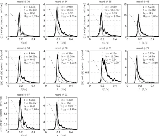
The compound effect of various wave conditions (mani- fested with various free surface elevation spectra in Fig. 1) and slightly varying z and h can be summarized with the value of L_E being the linear transfer function value at the frequency , the pressure gauge depth z and the water depth h . Obviously, as a single linear model can not be expected to cover that range of wave conditions as well as pressure and water depth variability, as caling factor based on L_E value will be used to improve accuracy of simula- tion. To show the variations in wave conditions in greater detail, free-surface elevation and pressure spectra are pre- sented in Fig. 1 together with linear transfer function L(f) which might be interpreted as the first approximation to fre- quency response of the system. Note, that although usually , the L(f) curves in Fig. 1 are scaled up by a maximum value of spectrum to show how the peak energy of the is transformed into p(t).

λ_TE

T_E^–1

L f( )∈[0 1, ]

ξ t( ) ξ t( )

Fig. 1. Free-surface elevation (bold line), wave pressure (thin line) spectra and linear transfer function L(f) (dash-dotted line). Non-dimen- sional L(f) is scaled to maximum of free surface elevation spectrum. p(t) scaled down and expressed in [m].

4. Application of SI techniques

In this section, techniques presented in section 2 are used to construct two distinct models: one referred to as free-sur- face model for simulating free-surface elevation using wave pressure as an input whereas the second one, referred to as wave pressure model will use free-surface elevation to simulate wave pressure. Despite working in opposite direc- tion both pressure and free-surface models share the same structure of ARX model presented in (7)~(9) with single output, multiple inputs and A = 1. The A operator polyno- mial is reduced to identity expressing the fact that y(t) at time t does not depend on its previous values but depends {y(t_p), t_p<t} on past and present values of input Q(t). As both models share also the structure of input vector Q(t), they will be presented jointly.

Data preprocessing included standard quality check proce- dures and high-frequency noise removal eliminating frequen- cies higher than 0.7 Hz (periods shorter than 1.3 s) using Butterworth anti-causal filter. The low-frequency part of records, which form an additional input in the sys- tem iden- tification technique described below, is defined as containing frequencies lower 0.03 Hz (periods longer than 30 s).

As stated in section 2, for efficient model estimation, the choice of model orders, time delays and input vectors is crucial. Delays of both models were set to zero due to reported fast instruments response and the nature of mod- elled system. Polynomial A was set to identity to provide greater stability with no loss on modelling accuracy com- paring to, for example, models with , which might be attributed to the high correlation between input an dout put of the system.

Construction of input vector and model orders, in turn, resulted from an iterative search for the best wave pressure model with sample data containing one elevation-pressure set and various input structures considered. Best results were achieved with an input vector consisting of free-sur- face elevation ,its square and low frequency

component that is: . The

free-surface elevation square proved to be especially useful incase of wave kinematics (Cielikiewicz and Gudmestad, 2001 and 2002) whereas the low frequency component was found to improve the performance of pressure models pro- vided model rank in was sufficiently high. The input structure determined during the tests was used in both mod- els. Furthermore, the test indicated that a dedicated model emphasizing the low frequency behavior might be useful.

Obviously, when estimation and validation data are distinct parts of the same series (i.e. p(t) and ξ(t) are divided into two separate estimation and validation parts), the simula- tion results on validation input are better than those achieved with the linear transfer function (LTF) method.

4.1. General model structure

In this paper, an estimated pressure or free-surface eleva- tion model is supposed to perform for similar values of z, h, and wave conditions with possible improvement achieved by simple rescaling of simulated time series. Taking into account the previously reported importance of low-fre- quency component, both the free-surface elevation and the pressure models will consist of two separate models: one for medium-frequency range G_M and another for low-fre- quency range G_L to form model output Y(t) as a sum:

(13)

Both G_M and G_L were estimated independently with:

and ; (14)

and ; (15)

where u(t) =ξ(t), u_L(t) =ξ_L(t) and t_M= p_M(t) in case of wave pressure model and u(t) = p(t), u_L(t) = p_L(t) and y_M=ξ_M(t) in case of free-surface elevation model. Note, that because of low frequency separation, data with ·_M subscript contain no low frequency component as it is modelled using its own model G_L. The ·_L subscript denotes low-frequency part of the series. All models share the same structure of an autoregres- sive model with extra input (ARX) outlined in (7)~(9) with

model orders , for main models G_M

and N_A= 1, N_B= [80] for the low frequency models G_L. As observed in Fig. 1, linear transfer function L(f) describes the amount of ξ(t) spectral energy transferred to pressure time series p(t) as predicted by linear theory. As the ARX coefficients are determined using narrow-band wave and pressure data, an ARX model, as applied in this study, is not likely to transfer reliably another free-surface elevation into pressure series if its spectrum is far from the spectral band of original data used to estimate the model. It was found that a simple linear scaling of modelled pressure by a ratio of transfer function values L_E for energy wave period improved results for almost all simulated pressure time series. The coefficient to multiply i^th simulated pres- N_A=10

ξ t( ) ξ t( )²

ξ_L( )t Q t( )=[ξ t( ) ξ t, ( )²,ξ_L( )t ]

ξ t( )

Y t( ) G= _M{Q_M( )t } G+ _L{Q_L( )t }

Q_M( )t =[u t( ) u t, ( )²,u_L( )t ] Y_M=[ ]y_M Q_L( )t =[u_L( )t ] Y_L=[ ]y_L

N_A=1 N_B =[80 80 80, , ]

sure time series takes the form of:

(16)

where index ·_e refers to record used for estimation. It is not clear whether scaling should be done using mean energy wave period T_E, peak wave period or mean wave period T_m01, but improvements over simulated p(t) were good enough in case of T_E. Unfortunately, for free-surface model, an equally good coefficient could not be found easily.

Wave pressure and free surface elevation models were esti- mated using the free surface elevation and pressure record

#38 and validated against the records 30, 34, 46, 50, 58, 61, 75, 87, 91. All pressure data except for the last two records come from the upper pressure transducer as described in sec- tion 3 and refer to the roughly the same transducer depth which is around 4 m in water depth of 16.0~16.8 m. No sig- nificant improvement was achieved by including any other pressure-elevation set into estimation data.

5. Results

As previously stated, both free-surface and wave pres- sure ARX models were validated using data collected under slightly different wave conditions manifested in record description in Table 1 and with varying spectra in Fig. 1.

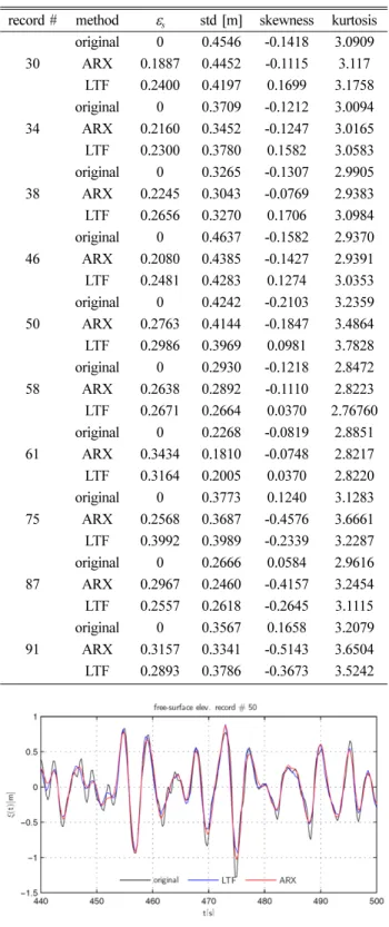
Simulation quality was measured using the scatter index _εs between simulated and original data for both ARX and LTF methods and by examination of the standard deviation, skewness and kurtosis with values listed in Tables 2 and 3.

All the simulated time series were visually compared to original time series using scatterplots shown in Fig. 3 and 5.

5.1 Free-surface elevation simulation based on time series

Free-surface simulation assumed the ARX model struc- ture outlined in (7)~(9) and input signal structures defined in (14)~(15) with y_M and y_L in (14) interpreted as a medium- and low-frequency components of free-surface elevation time series.

A sample of free-surface elevation time series for the record #50 simulated with ARX and LTF is presented in Fig. 2. For this exemplary sample, the ARX simulation quality is slightly better than LTF. Generally, the quality of free-surface simulation is not very high, with scatter index (ε_s) values within the 18~27%. However, traditional LTF simulation does not provide better result sand on 5 out of 9

cases ARX simulation is better than LTF (series 30, 34, 46, 50 and 75). Higher εs values in case of series 91, 87 and 61 are naturally expected as these series were recorded under different wave conditions (compared to other records) as t_i 1 1

2--- L f(_Ei;z_i,h_i) L f(_Ee;z_e,h_e) --- 1–

⎩ ⎭

⎨ ⎬

⎧ ⎫

+ 1 1

2--- L_Ei L_Ee --- 1–

⎝ ⎠

⎛ ⎞

+

= =

Table 2. Statistics of free-surface simulation using ARX and LTF compared with original data. Record # 38 (in bold) used for estimation

record # method εs std [m] skewness kurtosis original 0 0.4546 -0.1418 3.0909

30 ARX 0.1887 0.4452 -0.1115 3.117

LTF 0.2400 0.4197 0.1699 3.1758 original 0 0.3709 -0.1212 3.0094 34 ARX 0.2160 0.3452 -0.1247 3.0165 LTF 0.2300 0.3780 0.1582 3.0583 original 0 0.3265 -0.1307 2.9905 38 ARX 0.2245 0.3043 -0.0769 2.9383 LTF 0.2656 0.3270 0.1706 3.0984 original 0 0.4637 -0.1582 2.9370 46 ARX 0.2080 0.4385 -0.1427 2.9391 LTF 0.2481 0.4283 0.1274 3.0353 original 0 0.4242 -0.2103 3.2359 50 ARX 0.2763 0.4144 -0.1847 3.4864 LTF 0.2986 0.3969 0.0981 3.7828 original 0 0.2930 -0.1218 2.8472 58 ARX 0.2638 0.2892 -0.1110 2.8223 LTF 0.2671 0.2664 0.0370 2.76760 original 0 0.2268 -0.0819 2.8851 61 ARX 0.3434 0.1810 -0.0748 2.8217 LTF 0.3164 0.2005 0.0370 2.8220 original 0 0.3773 0.1240 3.1283 75 ARX 0.2568 0.3687 -0.4576 3.6661 LTF 0.3992 0.3989 -0.2339 3.2287 original 0 0.2666 0.0584 2.9616 87 ARX 0.2967 0.2460 -0.4157 3.2454 LTF 0.2557 0.2618 -0.2645 3.1115 original 0 0.3567 0.1658 3.2079 91 ARX 0.3157 0.3341 -0.5143 3.6504 LTF 0.2893 0.3786 -0.3673 3.5242

Fig. 2. A sample of ARX (red) and LTF (blue) simulated free-sur- face elevation #50 versus original data (black).

manifested with linear transfer function values L_E in Tables 1 and 2. Kurtosis and skewness are also reproduced better using ARX simulation. Furthermore, under typical (that is similar to those of estimation data) wave conditions ARX simulation seems to perform better at extreme values, which might be seen on scatterplots in Fig. 3.

5.2 Wave pressure simulation based on free-surface elevation time series

In this section wave pressure models were estimated assuming ARX structure outlined in (7)~(9) with output and input signal structures defined in (14)~(15). Naturally, in this case, y_M and y_L in (14) should be interpreted as the medium- and low-frequency components of wave pressure p(t) time series, respectively. As previously, the simulation quality was assessed with simple statistics and scatterplots as an overall performance indicators.

A sample of ARX and LTF simulated wave pressure time series can be observed in Fig. 4. This sample (record #50)

Fig. 3. Scatterplots of free surface simulated with ARX and LTF against original data. Record #38 used for ARX model estimation, rest of data provides validation.

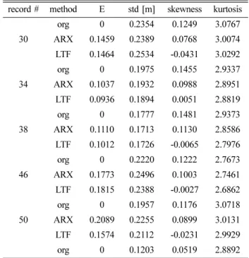
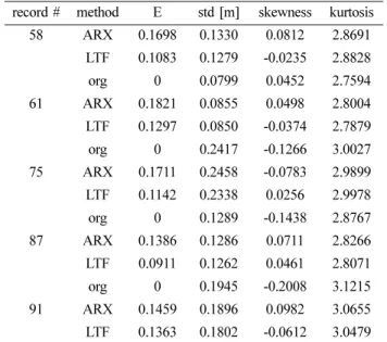
Table 3. Statistics of free-surface simulation using ARX and LTF compared with original data. Record #38 (in bold) used for estimation

record # method E std [m] skewness kurtosis

org 0 0.2354 0.1249 3.0767

30 ARX 0.1459 0.2389 0.0768 3.0074

LTF 0.1464 0.2534 -0.0431 3.0292

org 0 0.1975 0.1455 2.9337

34 ARX 0.1037 0.1932 0.0988 2.8951

LTF 0.0936 0.1894 0.0051 2.8819

org 0 0.1777 0.1481 2.9373

38 ARX 0.1110 0.1713 0.1130 2.8586

LTF 0.1012 0.1726 -0.0065 2.7976

org 0 0.2220 0.1222 2.7673

46 ARX 0.1773 0.2496 0.1003 2.7461

LTF 0.1815 0.2388 -0.0027 2.6862

org 0 0.1957 0.1176 3.0718

50 ARX 0.2089 0.2255 0.0899 3.0131

LTF 0.1574 0.2112 -0.0231 2.9929

org 0 0.1203 0.0519 2.8892

was chosen to correspond with the time series presented in Fig. 2. Although, as observed in Table 3, scatter index ε_s val- ues of ARX simulations are much lower (10~20%), the LTF

method performs in most cases better. However, in most cases, the original skewness and kurtosis values are approxi- mated better under ARX than using LTF. In case of pressure simulation, the ARX performance is slightly weaker than the traditional LTF when the model is applied to input data refer- ring to slightly different wave conditions, pressure gauge, water depth and its output is verified against measured data.

Basically, simulating pressure records requires filtering out Table 3. Continued

record # method E std [m] skewness kurtosis

58 ARX 0.1698 0.1330 0.0812 2.8691

LTF 0.1083 0.1279 -0.0235 2.8828

org 0 0.0799 0.0452 2.7594

61 ARX 0.1821 0.0855 0.0498 2.8004

LTF 0.1297 0.0850 -0.0374 2.7879

org 0 0.2417 -0.1266 3.0027

75 ARX 0.1711 0.2458 -0.0783 2.9899 LTF 0.1142 0.2338 0.0256 2.9978

org 0 0.1289 -0.1438 2.8767

87 ARX 0.1386 0.1286 0.0711 2.8266

LTF 0.0911 0.1262 0.0461 2.8071

org 0 0.1945 -0.2008 3.1215

91 ARX 0.1459 0.1896 0.0982 3.0655

LTF 0.1363 0.1802 -0.0612 3.0479

Fig. 4. A sample of ARX (red) and LTF (blue) simulated wave pressure for record # 50 versus original data (black).

Fig. 5. Scatterplots of wave pressure simulated with ARX and LTF against original data. Record #38 used for ARX model estimation, rest of data provides validation.

energy in a relevant frequency band; the linear transfer func- tion is a natural solution for this case.

However, if both estimation and validation data are a dis- tinct part of the same time series (which ensures exactly the same meteorological conditions, z and h values), the perfor- mance of the ARX simulation is better.

6. Conclusions

System identification procedures were shown to be effi- cient in the modelling of free-surface records basing on wave pressure record, especially if a low frequency compo- nent is included as an additional input time series. This is due to the fact, that the low frequency oscillations are far less attenuated in deep water column than the high fre- quency components.

Satisfactory performance of SI techniques in low fre- quency behavior modelling and noise robustness make these methods a good alternative to the corrected LTF method, under the assumption of similar water depth, gauge depth and wave conditions, especially for free-surface sim- ulation. As the Local Polynomial Approximation method is reported to perform similarly to LTF in case of high noise- to-signal ratio, ARX simulation might be locally, when dealing with noisy field data, shown to perform better than LPA. As neither LFA nor LSA have been applied to the field data yet, those methods have not been investigated.

Acknowledgements

This study was partially funded by the project PROZA, which in part has been funded by the European Union under the Innovative Economy Programme contract No.

POIG.010301-00/140/08. The authors would like to thank dr Luigi Cavaleri of Institute of Marine Sciences, CNR for providing wave data records collected at the Acqua Alta platform located near Venice.

References

Barker, C. H. and Sobey, R. J. Nonlinear wave kinematics from pressure arrays. Ocean Wave Measurement and Analysis (1997), ASCE, 787-801.

Barker, C. H. and Sobey, R. J. (1996). Irregular wave kinematics from a pressure record. Coastal Engineering Proceedings, 1(25).

Bendat, J. S. (1998). Nonlinear system techniques and applications.

Bhattacharyya, S. and Selvam, R. P. (2003). Parameter identifica- tion of a large floating body in random ocean waves by reverse

miso method. Journal of Offshore Mechanics and Arctic Engi- neering, 125, 81.

Biesel, F. (1982). Second order theory of manometer wave mea- surement. Coastal Engineering Proceedings, 1(18).

Bishop, C. T. and Donelan, M. A. (1987). Measuring waves with pressure transducers. Coastal Engineering, 11(4), 309-328.

Cavaleri, L. (1973). Ondametro a resistenza-critica, miglioramenti e precisione ottenibile. CNR Tech. Report.

Cavaleri, L. (1979). An instrumental system for detailed wind wave study. Il Nuovo Cimento C, 2(3), 288-304.

Cavaleri, L. (1980). Wave measurement using pressure transducer.

Oceanologica Acta, 3(3), 339-346.

Cavaleri, L. (1999). The oceanographic tower acqua alta: More than a quarter of a century of activity. Nuovo cimento della Società italiana di fisica. C, 22(1), 1-111.

Cavaleri, L. and Zecchetto, S. (1987). Reynolds stresses under wind waves. Journal of Geophysical Research: Oceans (1978–

2012), 92(C4), 3894-3904.

Cheng-Han Tsai, F.-J. Y., Young, F.-J., Lin, Y.-C. and Li, H.-W.

(2001). Comparison of methods for recovering surface waves from pressure transducers. Ocean wave measurement and anal- ysis: proceedings of the fourth international symposium, WAVES 2001: September 2-6, 2001, San Francisco, California, American Society of Civil Engineers, 347.

Cielikiewicz, W. and Gudmestad, O. T. (2001). System identifica- tion techniques for the modelling of irregular wave kinematics.

ASCE.

Cielikiewicz, W. and Gudmestad, O. T. (2002). System identifica- tion techniques for prediction of fluid accelerations under irreg- ular waves based on free-surface elevation measurements.

ASME.

Faltinsen, O. (1993). Sea loads on ships and offshore structures. Cambridge university press.

Fenton, J. and Christian, C. (1989). Inferring wave properties from sub-surface pressure data. Ninth Australasian Conference on Coastal and Ocean Engineering, 1989: Preprints of Papers, Institution of Engineers, Australia, 382.

Fenton, J. D. (1986). Polynomial approximation and water waves.

Coastal Engineering Proceedings, 1(20).

Folsom, R. (1947). Sub-surface pressures due to oscillatory waves.

Transactions, American Geophysical Union, 28, 875-881.

Grace, R. A. (1970). How to measure waves. Ocean Industry, 5(2), 65-69.

Hashimoto, N., Mitsui, M., Goda, Y., Nagai, T. and Takahashi, T.

(1996). Improvement of submerged doppler-type directional wave meter and its application to field observations. Coastal Engineering Proceedings, 1(25).

Kuo, Y.-Y. and Chiu, Y.-F. (1994). Transfer function between wave height and wave pressure for progressive waves. Coastal Engi- neering, 23(1), 81-93.

Lee, D.-Y. and Wang, H. (1984). Measurement of surface waves from subsurface gage. Coastal Engineering Proceedings, 1(19).

Ljung, L. (1987). System identication: Theory for the user. Preniice

Hall Inf and System Sciencess Series, New Jersey, 7632.

Masashi, H.-m., Howrikawa, K. and Komori, S. (1966). Response characteristics op underwater wave gauge. Coastal Engineering Proceedings, 1(10).

Mulk, M. T. U. and Falzarano, J. (1994). Complete six-degrees-of- freedom nonlinear ship rolling motion. Journal of Offshore Mechanics and Arctic Engineering, 116, 191.

Nielsen, P. (1989). Analysis of natural waves by local approxima- tions. Journal of Waterway, Port, Coastal, and Ocean Engineer- ing, 115(3), 384-396.

Panneer Selvam, R. and Bhattacharyya, S. (2001). Parameter iden- tification of a compliant nonlinear sdof system in random ocean waves by reverse miso method. Ocean engineering, 28(9), 1199- 1223.

Seiwell, H. (1947). Investigation of underwater pressure records and simultaneous sea surface patterns. Transactions, American Geophysical Union, 28, 722-724.

Sobey, R. J. (1992). A local fourier approximation method for irregular wave kinematics. Applied Ocean Research, 14(2), 93- 105.

Soderstrom, T. and Stoica, P. 1989. System identication. Prentice

Hall Inter. Ltd.

Stansby, P., Worden, K., Tomlinson, G. and Billings, S. (1992).

Improved wave force classification using system identification.

Applied ocean research, 14(2), 107-118.

Tick, L. J. (1959). A non-linear random model of gravity waves. J.

Math. Mech, 8(5), 643-651.

Townsend, M. and Fenton, J. D. (1996). A comparison of analysis methods for wave pressure data. Coastal Engineering Proceed- ings, 1(25).

Tsai, C.-H., Huang, M.-C., Young, F.-J., Lin, Y.-C. and Li, H.-W.

(2005). On the recovery of surface wave by pressure transfer function. Ocean Engineering, 32(10), 1247-1259.

Wang, H., Lee, D.-Y. and Garcia, A. (1986). Time series surface- wave recovery from pressure gage. Coastal engineering, 10(4), 379-393.

원고접수일: 2013년 12월 3일 수정본채택: 2013년 12월 30일 게재확정일: 2013년 12월 30일