Land Cover Classification Map of Northeast Asia Using GOCI Data

1. Introduction

Information regarding land cover (LC) changes over time is essential for studying the functional and morpho-functional changes occurring in the global ecological, meteorological, and hydrological environments (Chen et al., 2015; Feddema et al., 2005;

Son and Kim, 2018).

Remote sensing has long been recognized as an effective tool for broad-scale LC mapping and as an effective tool for generating LC maps needed to understand human activity and the biogeographical diversity of the land surface (Chen et al., 2015; Zhang and Roy, 2017). As a result, a number of LC products, such as global-scale maps based on remote sensing data, have been developed with broad-scale resolution

Land Cover Classification Map of Northeast Asia Using GOCI Data

Sanghun Son

· Jinsoo Kim

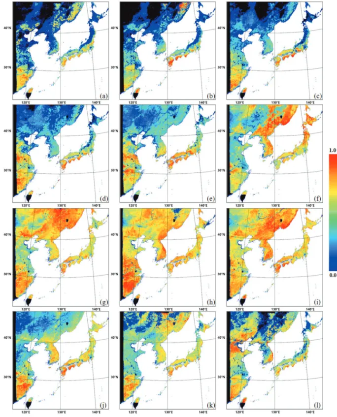
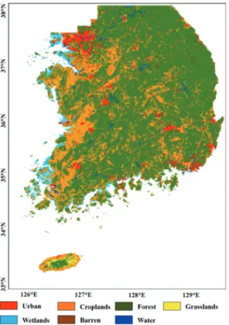
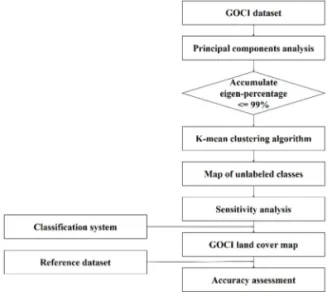
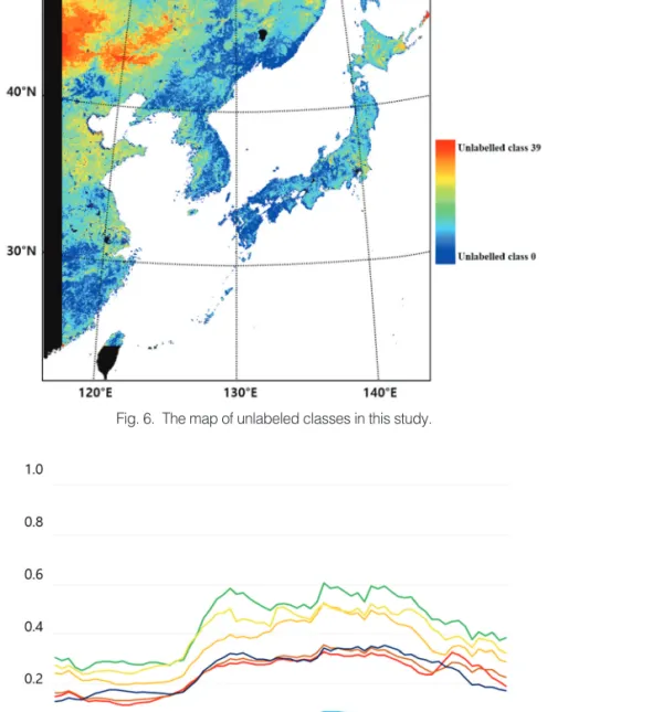
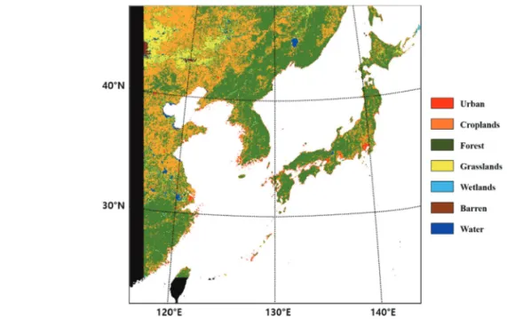
Abstract: Land cover (LC) is an important factor in socioeconomic and environmental studies. According to various studies, a number of LC maps, including global land cover (GLC) datasets, are made using polar orbit satellite data. Due to the insufficiencies of reference datasets in Northeast Asia, several LC maps display discrepancies in that region. In this paper, we performed a feasibility assessment of LC mapping using Geostationary Ocean Color Imager (GOCI) data over Northeast Asia. To produce the LC map, the GOCI normalized difference vegetation index (NDVI) was used as an input dataset and a level-2 LC map of South Korea was used as a reference dataset to evaluate the LC map. In this paper, 7 LC types (urban, croplands, forest, grasslands, wetlands, barren, and water) were defined to reflect Northeast Asian LC. The LC map was produced via principal component analysis (PCA) with K-means clustering, and a sensitivity analysis was performed. The overall accuracy was calculated to be 77.94%. Furthermore, to assess the accuracy of the LC map not only in South Korea but also in Northeast Asia, 6 GLC datasets (IGBP, UMD, GLC2000, GlobCover2009, MCD12Q1, GlobeLand30) were used as comparison datasets. The accuracy scores for the 6 GLC datasets were calculated to be 59.41%, 56.82%, 60.97%, 51.71%, 70.24%, and 72.80%, respectively. Therefore, the first attempt to produce the LC map using geostationary satellite data is considered to be acceptable.

Key Words: Land cover, Feasibility, Principal component analysis, K-means clustering, Overall accuracy Korean Journal of Remote Sensing, Vol.35, No.1, 2019, pp.83~92

https://doi.org/10.7780/kjrs.2019.35.1.6 ISSN 1225-6161 ( Print )

ISSN 2287-9307 (Online)

Article

Received January 31, 2019; Revised February 11, 2019; Accepted February 12, 2019; Published online February 18, 2019

1)

Master Student, Division of Earth Environmental System Science, Pukyong National University

2)

Assistant Professor, Department of Spatial Information Engineering, Pukyong National University

†

Corresponding Author: Jinsoo Kim ([email protected])

This is an Open-Access article distributed under the terms of the Creative Commons Attribution Non-Commercial License

(http://creativecommons.org/licenses/by-nc/3.0) which permits unrestricted non-commercial use, distribution, and reproduction in

any medium, provided the original work is properly cited.

through the efforts of many scientific communities (Arino et al., 2008; Bartholomé and Belward, 2005;

Bontemps et al., 2011; Friedl et al., 2002; Friedl et al., 2010; Hansen et al., 2000; Loveland and Belward, 1997; Loveland et al., 2000).

To date, several global land cover (GLC) datasets have been produced and widely applied in various fields. However, these datasets have different inputs, purposes of classification, classification methods, and classification systems (McCallum et al., 2006; Herold et al., 2008). Reported accuracies of GLC datasets range from 66% to more than 80% (Son and Kim, 2018). However, these GLC datasets have some drawbacks in Northeast Asia, especially in South Korea, due to insufficient validation data and misclassification. According to Park and Suh (2014), the Moderate Resolution Imaging Spectroradiometer (MODIS) LC dataset (MOD12Q1 and MCD12Q1), the most widely used GLC dataset in the world, have many misclassifications in Northeast Asia. Relevant input datasets, classification methods and classification systems are required to produce the LC map in Northeast Asia that appropriately reflects the Northeast Asia LC types.

All GLC datasets are produced using polar orbit satellite data. However, the disadvantage of polar orbit satellite imagery is that it is difficult to obtain data on the same region every day. On the other hand, geostationary satellites can obtain datasets over the same region every day. The purpose of this study is to assess the feasibility of LC mapping using Geostationary Ocean Color Imager (GOCI) data over Northeast Asia. The primary steps and contributions of this study are summarized as follows: (1) the principal component analysis (PCA) was based on using the GOCI normalized difference vegetation index (NDVI) to select principal components (PCs); (2) to produce an unlabeled map, the K-means clustering was conducted using PCs as input data; (3) through the sensitivity analysis, unlabeled classes were aggregated by LC type

and the LC map was produced; and (4) to analyze the feasibility of LC mapping, accuracy assessments were conducted using the reference dataset.

2. Data and Methodology 1) Study area and data

Fig. 1 shows the research area of this study that is composed of the Korean peninsula, Japanese Islands, and eastern part of China in Northeast Asia (latitude:

24.75–47.25°N, longitude: 113.4–146.6°E). This area is the same as the target area of the GOCI.

Datasets for the feasibility assessment of LC mapping using the GOCI data were divided in two: the first dataset consisted of the GOCI data as an input dataset to produce the LC map; the second dataset was the reference dataset to evaluate the LC map. The first dataset was composed of the GOCI NDVIs, which was calculated based on pre-processed bidirectional reflectance distribution function (BRDF) modeling for 16 days worth of data (Fig. 2). In addition, to minimize null values caused by clouds and snow, the second composite was based on the maximum value composite

Fig. 1. The research area of this study.

(MVC) over 7 days. To further minimize the effects of snow, the study period was selected to run from May 15, 2013 to October 15, 2013. The western and southern parts of the study area, which have null values

throughout the year, were masked for accurate LC mapping. The second dataset consisted of a level-2 LC map to assess the accuracy in South Korea (Fig. 3). In addition, to assess the accuracy of the LC map for LC

Fig. 2. GOCI NDVI used as an input dataset in this study, (a) Jan 16, (b) Feb 16, (c) Mar 16, (d) Apr 16, (e) May 16, (f) Jun

16, (g) Jul 16, (h) Aug 16, (i) Sep 16, (j) Oct 16, (k) Nov 16, (l) Dec 16.

types in Northeast Asia, we selected 6 GLC datasets (IGBP, UMD, GLC2000, GlobCover2009, MCD12Q1, and GlobeLand30) for Northeast Asia (Fig. 4). In order to produce accurate LC map, LC types that appropriately reflect the LC of Northeast Asia must be defined. GLC datasets that used widely in the world are IGBP, UMD, GLC2000, GlobCover2009, MCD12Q1. These Global land cover datasets have different classification system and 14 to 22 land cover types. In addition, the major classification system in the United States Geological Survey (USGS) defined 9 LC types (urban, croplands, grasslands, forest, water, wetlands, barren, tundra and permafrost). To name Northeast Asian land cover types, the number of land cover types in 5 GLC’s land cover types is not appropriate. Furthermore, among USGS`s land cover types, tundra and permafrost are not suitable land cover types in Northeast Asia. In this study, LC types were defined for 7 classes (urban, croplands, forest, grasslands, wetlands, barren, and water).

Fig. 4. 6 GLC dataset aggregated 7 classes used as comparison datasets. (a) IGBP, (b) UMD, (c) GLC2000, (d) GlobCover2009, (e) MCD12Q1, and (f) GlobeLand30.

Fig. 3. Level-2 LC map in South Korea with 7 classes used

as reference datasets.

2) Methodology

Fig. 5 shows a flow chart to assess the feasibility of LC mapping using the GOCI data over Northeast Asia. Input datasets for this study were composed of the GOCI NDVIs calculated via BRDF modeling.

BRDF modeling was calculated by proceeding to Eq.

(1) (Roujean et al., 1992).

R(θ

, θ

, ø) = K

+ K

· f

(θ

, θ

, ø) +

K

· f

(θ

, θ

, ø) (1) f

and f

denote the geometric kernel (Eq. (2)) and the volumetric kernel (Eq. (3)), respectively, and represent geometric scattering and volumetric scattering on the surface.

1 1 f

(θ

, θ

, ø) = —– [(π – ø) cos ø + sin ø] tan θ

tan θ

– —

2π π (2)

( ^{tan θ}

^{+ tan θ}

^{+ tan}

^θ

^{+ tan}

^θ

^{– 2 tan θ}

^{tan θ}

^{cos ø} )

4 1

f

(θ

, θ

, ø) = —– · ——————

3π cos θ

+ cos θ

(3) π 1 2 3 [( ^{— – ζ} ) cos ζ + sin ζ ] ^{– —}

ζ = arccos [cos θ

cos θ

+ sin θ

sin θ

cos ø] (4) According to Knight et al. (2006), differences in water levels over time lead to incorrect reflectance of infrared and red wavelengths at water–land boundaries and, depending on the turbidity and depth of the water,

the reflectance of infrared can have different values. In addition, it is difficult to spectrally differentiate between urban areas, suburban areas, grass cover, barren soil, and fallow areas (Lee and Lathrop, 2006). Therefore, to produce accurate the LC map, urban areas and water were masked in this study using GlobeLand30 and level-2 LC maps of South Korea. To select valuable data, input datasets were produced using PCA. In this study, we defined the PCs with an accumulated percentage of 99% or less. These PCs were used as input data for the K-means clustering algorithm. The result of the K-means clustering algorithm is a map of unlabeled classes, which will become the LC map through the sensitivity analysis. The last step is an accuracy assessment of the LC map using the reference dataset.

PCA is a multivariate technique used to reduce large datasets. The goal of PCA is to extract the valuable data, called PCs, from the dataset. PCA is commonly used as a data reduction technique in order to determine a new dataset of orthogonal variables having minimum dimensions ordered by variance (Han et al., 2004; Adbi and Williams, 2010). The results of the PCA consist of eigenvalues, eigen-percentages, and PCs, and the parameter of the PCA is the accumulated eigen- percentage. In this study, to select the most valuable data, the value of the accumulated eigen-percentage was less than 99% of an input dataset.

The K-means clustering is one of the most popular clustering techniques of unsupervised classification (Kanungo et al., 2000; Han et al., 2004). The K-means clustering is a data relocation technique that minimizes the distance between the centroid and dataset centered on initial centroids and determines n-datasets as k-clusters (Kim, 2002). The parameters, including number of classes, iteration, and threshold, must be specified in order to process the K-means clustering algorithm. The parameters of this study were determined empirically; 40 number of classes, 100 iterations, 0.95 threshold, 100 batch size, and 0 seeds.

Fig. 5. The flow chart in this study.

3. Results and discussion

The result of the K-means clustering algorithm is a map of unlabeled classes. In this study, the initial number of classes was 40 and Fig. 6 shows a map of unlabeled classes in this study. The high NDVI values were clustered into the blue area of the unlabeled map, and the low NDVI values were clustered into the red

area of the unlabeled map. In addition, the black part of the unlabeled map represents the masking area due to null values or urban and water masks.

Through the sensitivity analysis, these classes aggregate into LC types. In order to aggregate unlabeled classes, the NDVI time series of reference datasets were used as a comparison dataset (Fig. 7). The results of the NDVI time series of reference datasets

Fig. 7. The NDVI trends of the reference dataset used as a comparison data for the sensitivity analysis.

Fig. 6. The map of unlabeled classes in this study.

showed that the NDVI trend of forest areas was the highest, those of croplands and grasslands were similar, and those of urban, barren and water areas were lower than those of croplands and grasslands. The NDVI trend of wetland areas was lowest among all LC types.

Following the sensitivity analysis of the NDVI time series of the unlabeled map using the NDVI trends of reference dataset, the unlabeled classes aggregated to produce the LC map (Fig. 8). Table 1 presents a confusion matrix of the LC map and reference dataset.

In the case of cropland and forest areas, the LC types were well classified. However, grassland areas were overestimated. In addition, wetlands and barren areas were underestimated. Since urban and water areas were

masked, the overall accuracy was calculated based on 5 LC types (croplands, forest, grasslands, wetlands, and barren areas). Since more than 90% of South Korean LC types are classified as croplands and forest, the overall accuracy was calculated as 77.94%.

To assess the feasibility of the LC map for LC types in Northeast Asia, an accuracy assessment was performed using 6 GLC datasets: IGBP, UMD, GLC2000, GlobCover2009, MCD12Q1, and GlobeLand30. As in the previous accuracy assessment, confusion matrices were used to evaluate the LC map in Northeast Asia.

Table 2 shows the confusion matrices of 6 GLC datasets compared to the LC map. The overall accuracies compared to IGBP, UMD, GLC2000, GlobCover2009,

Fig. 8. The LC map with 7 classes in Northeast Asia.

Table 1. Confusion matrix of the LC map and reference dataset Reference dataset

Croplands Forest Grasslands Wetlands Barren Total

Croplands 56,277 23,990 1,470 540 517 82,794

Forest 37,027 225,414 3,488 240 511 266,680

Grasslands 8,174 2,685 295 497 429 12,080

Wetlands 131 49 7 70 6 263

Barren 49 13 0 13 3 78

Total 101,658 252,151 5,260 1,360 1,466 361,895

Overall accuracy (%) 77.94

MCD12Q1, and GlobeLand30 were calculated to be 59.41%, 56.82%, 60.97%, 51.71%, 70.24%, and 72.80%, respectively. The overall accuracies of MCD12Q1, the most widely used dataset in the world, and GlobeLand30, the best spatial resolution and the most recent land cover map, were calculated more than 75%.

4. Conclusions

LC is one of the major factors used to study global biogeochemical, meteorological, and hydrological characteristics. The goal of this paper was to produce an LC map using the GOCI data and to assess the feasibility of LC mapping using geostationary satellite data. First, to produce the LC map, the GOCI NDVIs was made through BRDF modeling and a level-2 LC map in South Korea was used as a reference dataset to assess the LC map. The LC map was produced as follows: (1) PCA was based on using the GOCI NDVIs to select PCs; (2) to produce an unlabeled map, the K- means clustering was conducted using PCs as input data; (3) through the sensitivity analysis, unlabeled classes were aggregated by LC type and the LC map was produced; and (4) to analyze the feasibility of LC mapping, accuracy assessments were conducted using the reference dataset. The overall accuracy compared with the reference dataset was calculated to be 77.94%.

In addition, the overall accuracies compared to IGBP, UMD, GLC2000, GlobCover2009, MCD12Q1, and GlobeLand30 were calculated to be 36.01%, 73.59%, 67.38%, 57.99%, 75.51%, and 77.59%, respectively.

In conclusion, LC mapping using the geostationary satellite data over Northeast Asia is considered to be a feasible mapping method.

Acknowledgements

This research was a part of the project titled

“Development of LC products for GOCI-II(C-D- 2018-0217)” funded by the Ministry of Oceans and Fisheries, Korea and this work was supported by the BK21 plus Project of the Graduate School of Earth Environmental Hazard System.

References

Abdi, H. and L.J. Williams, 2010. Principal component analysis, WIREs Computational Statistics, 2(4):

433-459.

Arino, O., P. Bicheron, F. Achard, F. Latham, R. Witt, and J.L. Weber, 2008. GLOBCOVER–the most detailed portrait of Earth, European Space Agency Bulletin, 136: 25-31.

Bartholomé, E. and A. S. Belward, 2005. GLC2000: a new approach to global land cover mapping from Earth observation data, International Journal of Remote Sensing, 26(9): 1959-1977.

Bontemps, S., P. Defourny, E.V. Bogaert, O. Arino, V. Kalolgirou, and J.R. Perez, 2011.

GLOBCOVER 2009 Products Description and Validation Report, European Space Agency, Paris, France.

Chen, J., J. Chen, A. Liao, X. Cao, L. Chen, X. Chen, C. He, G. Han, S. Peng, M. Lu, W. Zhang, X.

Tong, and J. Mills, 2015. Global land cover mapping at 30 m resolution: A POK-based operational approach, ISPRS Journal of Photogrammetry and Remote Sensing, 103:

7-27.

Table 2. The overall accuracies of the 6 GLC maps

IGBP UMD GLC2000 GlobCover2009 MCD12Q1 GlobeLand30

Overall accuracy

(%) 59.41 56.82 60.97 51.71 70.24 72.80

Feddema, J.J., K.W. Oleson, G.B. Bonan, L.O. Mearns, L.E. Buja, G.A. Meehl, and W.M. Washington, 2005. The importance of land-cover change in simulating future climates, Science, 310 (575409): 1674-1678.

Friedl, M.A., D. Sulla-Menashe, B. Tan, A. Schneider, N. Ramankutty, A. Sibley, and X. Huang, 2010. MODIS collection 5 global land cover:

algorithm refinements and characterization of new datasets, Remote Sensing of Environment, 114(1): 168-182.

Friedl, M.A., D.K. McIver, J.C. Hodges, X. Zhang, D.

Muchoney, A.H. Strahler, C.E. Woodcock, S.

Gopal, A. Schneider, and A. Cooper, 2002.

Global land cover mapping from MODIS:

algorithms and early results, Remote Sensing of Environment, 83(1&2): 287-302.

Han, K.S., J.L. Champeaux, and J.L. Roujean, 2004. A land cover classification product over France at 1 km resolution using SPOT4/VEGETATION data, Remote Sensing of Environment, 92(1):

52-66.

Hansen, M.C., R.S. Defries, J.R.G. Townshend, and R. Sohlberg, 2000. Global land cover classification at 1 km spatial resolution using a classification tree approach, International Journal of Remote Sensing, 21(6&7): 1331-1364.

Herold, M., P. Mayaux, C.E. Woodcock, A. Baccini, and C. Schmullius, 2008. Some challenges in global land cover mapping: An assessment of agreement and accuracy in existing 1 km datasets, Remote Sensing of Environment, 112(5): 2538-2556.

Kanungo, T., D.M. Mount, N.S. Netanyahu, C. Piatko, R. Silverman, and A.Y. Wu, 2000. The analysis of a simple K-means clustering algorithm, Proc. of the sixteenth annual symposium on Computational geometry, Kowloon, Hong Kong, Jun. 12-14, pp. 100-109.

Kim, N.Y., H.J. Oh, D.U. An, and S.C. Park,

2002. Document clustering analysis based on similarity calculation between cluster centroids, The Institute of Electronics and Information Engineers, 25(2): 119-122 (in Korean with English abstract).

Knight, J.F., R.S. Lunetta, J. Ediriwickrema, and S.

Khorram, 2006. Regional scale land cover characterization using MODIS-NDVI 250 m multi-remporal imagery: A phenology-based approach, GIScience and Remote Sensing, 43(1): 1-23.

Lee, S. and R.G. Lathrop, 2006. Subpixel analysis of Landsat ETM + using Self-Organizing Map (SOM) neural networks for urban land cover characterization, IEEE Transactions on Geoscience and Remote Sensing, 44(6):

1642-1654.

Loveland, T.R. and A.S. Belward, 1997. The IGBP-DIS global 1 km land cover data set, DISCover:

first results, International Journal of Remote Sensing, 18(15): 3289-3295.

Loveland, T.R., B.C. Reed, J.F. Brown, D.O. Ohlen, L.

Yang, and W. Merchant, 2000. Development of a global land cover characteristics database and IGBP DISCover from 1 km AVHRR data, International Journal of Remote Sensing, 21(6&7): 1303-1330.

McCallum, I., M. Obersteiner, S. Nilsson, and A.

Shvidenko, 2006. A spatial comparison of four satellite derived 1 km global land cover dataets, International Journal of Applied Earth Observation and Geoinformation, 8(4):

246-255.

Park, J.Y. and M.Y. Suh, 2014. Characteristics of MODIS land-cover data sets over Northeast Asia for the recent 12 years (2001-2012), Korean Journal of Remote Sensing, 30(4):

511-524 (in Korean with English abstract).

Roujean, J.L., M. Leroy, and P.Y. Deschamps, 1992.

A Bidirectional Reflectance Model of the

Earth’s Surface for the Correction of Remote Sensing Data, Journal of Geophysical Research, 97(D18): 20455-20468.

Son, S.H. and J.S. Kim, 2018. Accuracy assessment of global land cover datasets in South Korea, Korean Journal of Remote Sensing, 34(4):

601-610.

Zhang, H.K. and D.P. Roy, 2017. Using the 500 m

MODIS land cover product to derive a

consistent continental scale 30 m Landsat

land cover classification, Remote Sensing of

Environment, 197: 15-34.