https://doi.org/10.7848/ksgpc.2017.35.4.241
Accuracy Improvement of KOMPSAT-3 DEM Using Previous DEMs without Ground Control Points
Lee, Hyoseong1)·Park, Byung-Wook2)·Ahn, Kiweon3)
Abstract
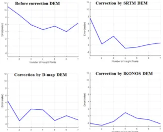
GCPs (Ground Control Points) are needed to correct the DEM (Digital Elevation Model) produced from high- resolution satellite images and the RPC (Rational Polynomial Coefficient). It is difficult to acquire the GCPs through field surveys such as GPS surveys and to read the image coordinates corresponding to the GCPs. In addition, GCPs cannot cover the entire image of the test site, and the RPC correction results may be influenced by the arrangement and distribution of the GCPs in the image. Therefore, a new method for the RPC correction is needed. In this study, an LHD (Least-squares Height Difference) DEM matching method was applied using previous DEMs: SRTM DEM, digital map DEM, and corrected IKONOS DEM. This was carried out to correct the DEM produced from KOMPSAT-3 satellite images and the provided RPC without GCPs. The IKONOS DEM had the highest accuracy, and the height accuracy was about ± 3 m RMSE in a mountainous area and about ± 2 m RMSE in an area with only low heights.
Keywords : RPC, LHD DEM Matching, SRTM DEM, Digital Map DEM, IKONOS DEM
241 Original article
1. Introduction
KOMPSAT-3’s RPC is generated from a physical sensor model, but it contains positioning error (Lee et al., 2013).
GCPs are needed to correct the DEM produced from high- resolution satellite images and the RPC. However, it is difficult to acquire GCPs through field surveys such as GPS surveys and to read the image coordinates corresponding to the GCPs. In addition, GCPs cannot cover the entire image of the test site, and the RPC correction results may be influenced by the arrangement and distribution of the GCPs in the image.
Previous works have attempted to use a set of reference data such as DEM, LiDAR, and digital map data instead of GCPs. Since these can be secured as control points in the entire image and do not require field work, it is possible to improve the RPC accuracy efficiently and conveniently and to
automate the process (Oh and Jung, 2012; Lee and Oh, 2014;
Oh and Lee, 2014). Oh and Jung (2012) proposed a method for automatically correcting the RPC of KOMPSAT-2 by using SRTM DEM. Lee and Oh (2014) proposed the RECC (Relative Edge Cross Correlation) method for image matching, and corrected the RPC of KOMPSAT-2 and KOMPSAT-3 satellite images. However, since these are basically matching techniques using feature points of image pixel values, only two-dimensional transformation parameters such as the affine transform, and the height is not considered. Therefore, such methods are not suitable for the required three-dimensional transform parameters (translation, rotation, scale) between two DEMs, and the transformed three-dimensional coordinates are also inaccurate.
To solve this problem, a DEM matching method can be used. Such a method corrects the orientation of the object
This is an Open Access article distributed under the terms of the Creative Commons Attribution Non-Commercial License (http://
creativecommons.org/licenses/by-nc/3.0) which permits unrestricted non-commercial use, distribution, and reproduction in any medium, provided the original work is properly cited.
Received 2017. 07. 13, Revised 2017. 08. 18, Accepted 2017. 08. 28
1) Member, Dept. of Civil Engineering, Sunchon National University (E-mail: [email protected])
2) Corresponding Author, Member, Dept. of Civil, Safety, and Environmental Engineering, Hankyong National University (E-mail: [email protected]) 3) Member, Dept. of Civil Engineering, Gyeongsang National University (Engineering Research Institute) (E-mail: [email protected])
Journal of the Korean Society of Surveying, Geodesy, Photogrammetry and Cartography, Vol. 35, No. 4, 241-248, 2017
DEM, which is generated from an initial sensor model (e.g., the exterior orientation parameter or RPC) after obtaining the three-dimensional transform parameters between the object DEM and the reference DEM. One of the popular methods is the ICP (Iterative Closest Point) method. This method is based on the point-to-point or point-to-plane searching techniques and an estimation of the rigid transformation that aligns the pairs of nearest points in two datasets (Gruen and Akca, 2005). It is also widely used for real-time location measurements of robots in the computer vision field (Besl and McKay, 1992; Joung, 2009). However, this method may be distorted between DEMs that have a certain pattern of shapes or only partial overlapping. In addition, it requires many iterations and much time to find the same point (Gruen and Akca, 2005; Han, 2007).
Another approach to match two DEMs is the LHD technique, which is based on the height difference of the same plane position between two DEMs for an absolute orientation of the frame sensor (Rosenholm and Torlegård, 1988; Ebner and Strunz, 1988). Kim and Jeong (2011) proposed an extension method of the LHD technique for application to the absolute orientation of a satellite image with a pushbroom sensor. The LS3D (Least-Squares 3D) surface matching method was also developed using three-dimensional surface shapes (Gruen and Akca, 2005). In addition DEM matching can be used for comparison or change analysis of DEMs from different periods in the same area (Karras and Petsa, 1993;
Zhang et al., 2005; Lee et al., 2011).
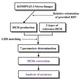
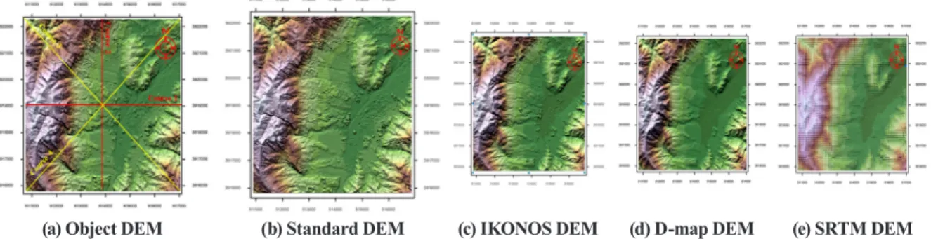
In this study, we used the LHD DEM matching method using reference DEMs to correct an object DEM produced by the provided RPC of KOMPSAT-3 satellite images. The reference DEMs consist of SRTM DEM, DEM by a 1:5,000 Digital-map (D-map DEM), and DEM from IKONOS satellite images and the corrected RPC with GCPs (IKONOS DEM). We determined the most suitable reference DEM and present the accuracy for the LHD technique.
2. DEM Matching Algorithm Using Least- squares Height Difference
The flow of the study is shown in Fig. 1. The 3D similarity transformation (Eq. 1) was used to correct the produced
DEM from the RPC provided. The DEM can be corrected by using seven calculated parameters (three translations, three rotational angles, and a scale):
′′
′
′′
′
( and ) å
(e.g., ∆ ),
′ ′′
′ ′ ′ ′ ′′
() () ( ⋯ )
⋯
(1) where X, Y and Z are 3-D coordinates of the reference DEM;
′′
′
′ ′
′
( and ) å
(e.g., ∆ ),
′ ′ ′
′ ′ ′ ′ ′ ′
() ()
( ⋯ )
⋯
,
′′
′
′ ′
′
( and ) å
(e.g., ∆ ),
′ ′ ′
′ ′ ′ ′ ′ ′
() ()
( ⋯ )
⋯
and
′′
′
′ ′
′
( and ) å
(e.g., ∆ ),
′ ′ ′
′ ′ ′ ′ ′ ′
() ()
( ⋯ )
⋯
are the 3-D coordinates of the object DEM. X, Y and
′′
′
′ ′
′
( and ) å
(e.g., ∆ ),
′ ′ ′
′ ′ ′ ′ ′ ′
() ()
( ⋯ )
⋯
,
′′
′
′ ′
′
( and ) å
(e.g., ∆ ),
′ ′ ′
′ ′ ′ ′ ′ ′
() ()
( ⋯ )
⋯
are the same plane coordinates, while Z and
′′
′
′ ′
′
( and ) å
(e.g., ∆ ),
′ ′ ′
′ ′ ′ ′ ′ ′
() ()
( ⋯ )
⋯
are different heights.
′′
′
′ ′
′
( and ) å
(e.g., ∆ ),
′ ′ ′
′ ′ ′ ′ ′ ′
() ()
( ⋯ )
⋯
,
′′
′
′ ′
′
( and ) å
(e.g., ∆ ),
′ ′ ′
′ ′ ′ ′ ′ ′
() ()
( ⋯ )
⋯
and
′′
′
′ ′
′
( and ) å
(e.g., ∆ ),
′ ′ ′
′ ′ ′ ′ ′ ′
() ()
( ⋯ )
⋯
are translations, S is a scale factor, R is an orthogonal rotation matrix that contains rotational angles (
′′
′
′ ′
′
( and ) å
(e.g., ∆ ),
′ ′ ′
′ ′ ′ ′ ′ ′
() ()
( ⋯ )
⋯
,
′′
′
′ ′
′
( and ) å
(e.g., ∆ ),
′ ′ ′
′ ′ ′ ′ ′ ′
() ()
( ⋯ )
⋯
and
′′
′
′ ′
′
( and ) å
(e.g., ∆ ),
′ ′ ′
′ ′ ′ ′ ′ ′
() ()
( ⋯ )
⋯
) with respect to the X, Y and Z, respectively.
Eq. 1 can be linearized by Taylor series expansion as shown in Eq. 2 based on the theory from Rosenholm and Torlegård (1988).
′′
′
′ ′
′
( and ) å
(e.g., ∆ ),
′ ′ ′
′ ′ ′ ′ ′ ′
() ()
( ⋯ )
⋯
can be computed by the least squares method and iteration (e.g.,
′′
′
′ ′
′
( and ) å
(e.g., ∆ ),
′ ′ ′
′ ′ ′ ′ ′ ′
() ()
( ⋯ )
⋯
), and the seven parameters are determined until the variables of the terms
′′
′
′ ′
′
( and ) å
(e.g., ∆ ),
′ ′ ′
′ ′ ′ ′ ′ ′
() ()
( ⋯ )
⋯
are close to zero.
′′
′
′ ′
′
( and ) å
(e.g., ∆),
′′ ′
′ ′ ′ ′ ′′
() () (⋯ )
⋯
(2) where
′′
′
′ ′
′
( and ) å
(e.g., ∆ ),
′ ′ ′
′ ′ ′ ′ ′ ′
() ()
( ⋯ )
⋯
is the initial height value calculated by the initial seven parameters and
′′
′
′ ′
′
( and ) å
(e.g., ∆ ),
′ ′ ′
′ ′ ′ ′ ′ ′
() ()
( ⋯ )
in the term Z in Eq. (1), and
′′
′
′ ′
′
( and ) å
(e.g., ∆ ),
′ ′ ′
′ ′ ′ ′ ′ ′
() ()
( ⋯ )
⋯
and
′′
′
′ ′
′
( and ) å
(e.g., ∆ ),
′ ′ ′
′ ′ ′ ′ ′ ′
() ()
( ⋯ )
⋯
are the slopes with respect to the X and Y directions of the two grid spaces in the object DEM.
Fig. 1. Flow chart for DEM matching and DEM correction