2004, Vol. 15, No. 4, pp. 911∼920
Receiver Operating Characteristic (ROC) Curves Using Neural Network in Classification
1)Jea-Young Lee2) ⋅ Yong-Won Lee3)
Abstract
We try receiver operating characteristic(ROC) curves by neural networks of logistic function. The models are shown to arise from model classification for normal (diseased) and abnormal (nondiseased) groups in medical research. A few goodness-of-fit test statistics using normality curves are discussed and the performances using neural networks of logistic function are conducted.
Keywords : Activation function, Logistic regression, Neural networks, Receiver operating characteristic (ROC) curve
1. Introduction
A logistic regression analysis may belong to one of many techniques for classification that divide data into the normal group(diseased) and the abnormal group(nondiseased) in medical research. Specially, in neural networks it is easy to accept but difficult to use the results from a classification because the analysis process is greatly complicated and hidden. Using the special quality of the activation function concerned deeply in output result of the neural network analysis, we apply the results of neural networks for a classification in data mining to the ROC logistic modelling.
On the other hand, there are graphical methods for doing normality test such as Q-Q (quantile-quantile) plot and P-P(probability-probability) plot. Wilk and
1) This research was supported by the Yeungnam University research grants in 2002 2) First Author : Professor, Department of Statistics Yeungnam University Kyongsan,
Kyongbuk, 712-749 Korea E-Mail : [email protected]
3) Graduate, Department of Statistics Yeungnam University Kyongsan, Kyongbuk, 712-749 Korea
Granadesikan (1968) introduced probability plotting methods for the analysis of data and normality test. Mage(1982) introduced some graphical methods for normality test. Lee, Woo and Rhee (1998) proposed a new graphical method named a transformed quantile-quantile plot to test for normality. However graphical method is less formal and the use of it alone could lead to a spurious conclusion.
To solve this kind of problem, Lee and Rhee(1999) proposed the goodness-of-fit test for normality through ROC analysis. They obtained the estimated sample variances, S2QQ and S2PP from residuals of the transformed Q-Q and the transformed P-P plots respectively. Also the comparisons with Shapiro and Wilk's W statistic (1965), were conducted by Monte Carlo simulations. This paper is organized as follows. Section 2 describes two statistics, the estimated sample variances, S2QQ and S2PP from P-P and Q-Q plots, respectively, ROC curves and their statistical performances. Section 3 considers a method of neural networks for classification in data mining and suggests a ROC curves for normal(diseased) and abnormal(nondiseased) groups by neural networks. Further, a simulation studies and comparisons are discussed. The final section is devoted to summary.
2. The Estimated Sample Variances of Q-Q, P-P Plots and ROC Curves
The Q-Q(quantile-quantile) plot and P-P(probability-probability) plots are well-known graphical methods for normality test. The goodness-of-fit test of normality by ROC curves are discussed by Lee & Rhee(1999). That is, the estimated sample variance, S2QQ, from residuals of the TQQ plot.
S2QQ = 1 n - 1 ∑
n
i = 1
{
Φ- 1(
n - 2c + 1i - c)
- xi:n}
2= 1
n - 1 Ln, c∈[ 0, 1 ) ,
where Ln = ∑
n
i = 1
{
Φ- 1(
n - 2c + 1i - c)
- xi:n}
2 with c = 0 (DeWet and Venter, 1972). and Φ is a cumulative function of standard normal distribution.The estimated sample variance, S2PP, from residuals of the transformed TPP plot is obtained by
S2 PP= 1 n - 1 ∑
n
i = 1
{ ( ni - n + 1n ×Φ( xi:n))
- n1 ∑nj (
nj - n + 1n ×Φ( xj:n)) }
2
Receiver operating characteristic(ROC) curve analysis was developed to summarize data from signal detection experiments in psychophysics(Green and Swets,1966). Recently, ROC curves are used to evaluate diagnostic tests when test results are not binary. In biomedical applications, the two states are often referred to as diseased and nondiseased, or D+ and D- for short. Central to this analysis is the ROC curve, which displays diagnostic accuracy as a series of pairs of performance measures. Each pair consists of a true positive fraction(TPF) and the corresponding false positive fraction(FPF) for a given definition of test positivity.
In the medical literature, the term TPF is called sensitivity and the complement of the FPF is called specificity. They are simply defined as
Number of True Positive Decisions Sensitivity
Number of Actually Positive Cases
≡
Number of True Negative Decisions Specificity
Number of Actually Negative Cases
≡
The ROC curve is to plot in the series of the sensitivity(TPF) versus [1-specificity(FPF)] pairs. The area under the population ROC curve represents the probability that the resulting values will be in the correct order when the variable is observed for a randomly selected individual from the abnormal population and for a randomly selected individual from the normal population. So a more accurate test will be located on an ROC curve closer to the left top corner than a less accurate one. And accuracy is defined by
Number of Total Correct Decisions Accuracy
Number of Total Cases
Fraction of the Study Population Sensitivity
that is Actually Positive Fraction of the
Specificity
≡
= ×
+ ×
Study Population that is Actually Negative
Let D be a binary indicator of normal status such as 1, .
0, . diseased
D nondiseased
=
and let Ydenote the result of a nonbinary diagnostic test. For some threshold y,
test results greater than y, are assumed to be indicative of normal. Then the sensitivity and specificity associated with this decision criterion can be written as, respectively,
Sen( y) = Pr [Y ≥y | D = 1]
Spec( y) = Pr [Y < y | D = 0]
Suppose that a sample of N individuals undergo a test for predicting an event of interest or determining presence or absence of a medical condition and that the test is based on a continuous-valued diagnostic variable. We assume that higher values of the test variable are associated with the event of interest for convenience.
For the goodness-of-fit test of normality by ROC areas, we use these three statistics W, S2QQ and S2PP. A simulation study is conducted for various sample sizes where we consider alternative hypothesis exponential distribution (skewed distribution).
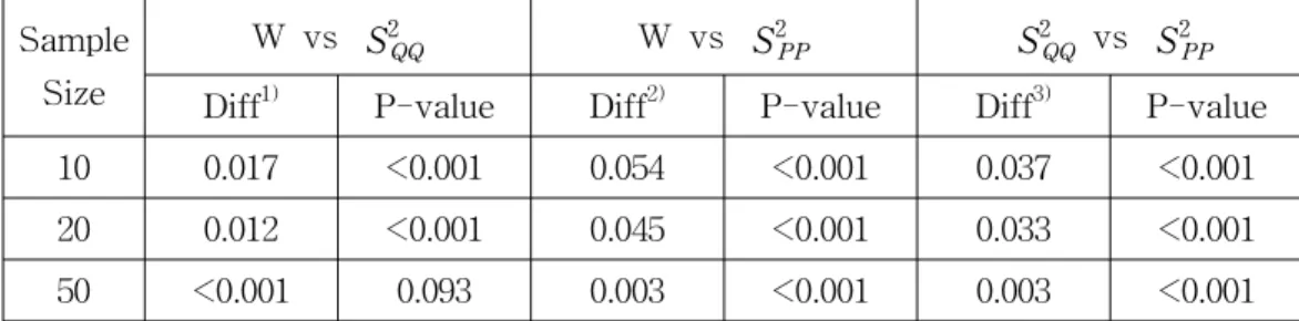
Table 2.1. Statistical Analysis between ROC Areas by W, S2PP and S2QQ statistics Sample
Size
W vs S2QQ W vs S2PP S2QQ vs S2PP
Diff1) P-value Diff2) P-value Diff3) P-value
10 0.017 <0.001 0.054 <0.001 0.037 <0.001
20 0.012 <0.001 0.045 <0.001 0.033 <0.001
50 <0.001 0.093 0.003 <0.001 0.003 <0.001
1) Diff = ROC Area of W - ROC Area of S2QQ, 2) Diff = ROC Area of W - ROC Area of S2PP, 3) Diff = ROC Area of S2QQ - ROC Area of S2PP
That is, we generate N=2,000 random W, S2QQ, and S2PP samples for each sample size n=10, 20, and 50. Then, Then, we gather N=4,000 random samples and order descending the total of random samples. To change the threshold y, we get some sensitivities and specificities. The empirical ROC curve is a plot of sens versus [1- spec]. So we apply those samples for the ROC curve and calculate the area under ROC curve. The results are summarized in Table 2.1 (Lee and Rhee, 1999).
Comparing ROC area and accuracy results, we see that W-statistic is typically superior to S2QQ and S2PP in detecting the skewed distribution (exponential distribution) for all sample sizes. Comparing S2QQ and S2PP, S2QQ dominates S2PP
for all sample sizes. Of course, all W, S2QQ and S2PP statistics have approximate 100 % ROC areas for a moderate or large sample sizes such as n =50. The results indicate W-statistic of three is the most suitable for testing normality, but
S2QQ statistic is also a comparative statistic.
3. ROC Curves by Neural Networks using Logistic Function of Sigmoidal Function
We consider only the classification problem about two classes such as the normal(diseased) group CN and the abnormal(nondiseased) group CA in medical research. Let the training data set be defined by
T ={ ( x( n),d( n)) | n = 1, 2, …, N} (3.1)
where x (n ) is a m-dimensional input vector for item n and N is the total number of cases or items used in this analysis. And d (n ) is a desired response or target output for item n such as
d (n ) =
1, x (n ) CA
0, x (n ) CN (3.2) In neural networks, the output of each node is made by the activation function.
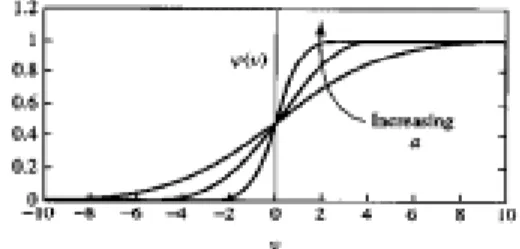
Specially, the model of each neuron in multilayer perceptron has a nonlinear and smooth activation function. A commonly used form of sigmoidal nonlinearity function is defined by a logistic function (Haykin,1999) such as
Φ(v) = 1
1 + exp- av (3.3) where a is the slope parameter of the sigmoid function.
In Figure 3.1, by varying the parameter a, sigmoid functions of different slopes are illustrated. The results of the activation function from the output layer (Figure 3.1) with a single node of a multilayer perceptron with the error back-propagation algorithm are often called by scores and denoted by O( n), n = 1, 2, …, N (Haykin, 1999). We calculate these scores using logistic function of sigmoidal function.
Hji= f1(b0+ wi×Zxi) , i = 1, 2, …, N, j = 1, 2, …, k
Where f1 is a logistic function, Hji is a score of jth hidden layer and ith observation, b0 is a bias, wi is a weight of ith observation and Zx
i is a normality of observation. We can change the number of hidden layers. Then, we take scores by
O( n) = ∑k
j = 1f2(b1+ wjHji) , i = 1, 2, …, N, j = 1, 2, …, k
Where f2 is a logistic function, b1 is a bias and wj is a weight of jth hidden layer.
Figure 3.1. Sigmoid activation function (Haykin,1999) These scores are characterized by
dˆ(n ) =
1, x (n ) CA
0, x (n ) CN (3.4)
where dˆ(n ) is the result of classification for item n and c is a constant. In the multilayer perceptron with the activation function which is equation (3.3), the range of O (n ) is [0, 1] and the constant c=0.5. Then the classification rules are following:
① If a score O (n ) is great than or equal to 0.5, then the item n is classed to the abnormal class CA.
② If a score O (n ) is less than 0.5, then the item n is classed to the normal class CN.
The scores have been used to classify by the classification rules(① and ②) only.
In statistical viewpoint, a final output dˆ(n )is the estimation of the desired response d (n ). That is, the event such as dˆ(n )=1 is equivalent to O (n ) c. So, the probability form is formulated by
P [dˆ(n ) = 1 ] = P [O (n ) c ] (3.5) and
P [dˆ(n ) = 0 ] = P [O (n ) < c ] (3.6) From (3.5) and (3.6), we define the survival distributions, which are defined sensitivity and 1-specificity respectively, of X of diseased and nondiseased populations such as
FD(x ) = P [X x|d = 1 ] (3.7) and
FD(x ) = P [X x|d = 0 ] (3.8)
The ROC curves by sensitivity(FD(x )) versus 1-specificity(F
D(x ) ) are tried and ROC Area by Neural Network Score were showed in Table 3.1. Also, ROC curve is defined by Pepe(1997) such as
ROC (t ) = FD(x ) = FD(F− 1
D (t )), t (0, 1 ) (3.9) where t is the false positive rate, that is, t = FD(x ) for all nonparametric areas(McNeil and Hanley, 1984) under ROC curves.
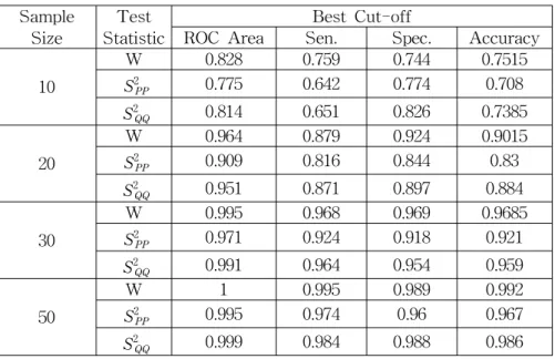
Table 3.1 ROC Areas by Neural Network Score Sample
Size
Test Statistic
Best Cut-off
ROC Area Sen. Spec. Accuracy
10
W 0.828 0.759 0.744 0.7515
S2PP 0.775 0.642 0.774 0.708
S2QQ 0.814 0.651 0.826 0.7385
20
W 0.964 0.879 0.924 0.9015
S2PP 0.909 0.816 0.844 0.83
S2QQ 0.951 0.871 0.897 0.884
30
W 0.995 0.968 0.969 0.9685
S2PP 0.971 0.924 0.918 0.921
S2QQ 0.991 0.964 0.954 0.959
50
W 1 0.995 0.989 0.992
S2PP 0.995 0.974 0.96 0.967
S2QQ 0.999 0.984 0.988 0.986
The results in Table 3.1, indicate that areas under ROC curves (ROC Area) for three normality statistics from obtained scores, O (n ). Comparing ROC area and accuracy results by neural networks, we see that W-statistic is typically superior to S2QQ and S2PP in detecting the skewed distribution (exponential distribution) for all sample sizes. Of course, all W, S2QQ and S2PP statistics have approximate 100
% ROC areas for a moderate or large sample sizes such as n =50. The results of neural networks indicate W-statistic is the more suitable for testing normality, but
S2QQ statistic is also a comparative statistic.
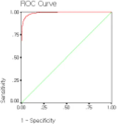
Figure 3.2. ROC Curve of W statistic by Neural Network at size 30
Figure 3.3. ROC Curve of SPP2 statistic by Neural Network at size 30
Figure 3.4. ROC Curve of SQQ2 statistic by Neural Network at size 30
Through figures 3.2 to 3.4 represent estimated ROC curves of three normality
statistics by neural network methods. Through these figures, we obtain that the ROC curves for Shapiro-Wilk W statistic are greater than others. But Q-Q plot's is also comparative. These results are discussed in Table 3.1. also.
4. Conclusions
ROC curves for normal and abnormal classifications is proposed using neural networks of data mining. By using two statistics SQQ2 and SPP2 of two graphical techniques(P-P and Q-Q plots) for normality, we compared with numerical technique(Shapiro-Wilk's W statistic). The results in Table 3.1, indicate that normality statistics W and SQQ2 are superior to SPP2 for all samples, but W and SQQ2 are comparative. So we may conclude that Q-Q plot's SQQ2 is as powerful as Shapiro-Wilk's W for the normality test.
Through Figures 3.2 to 3.4, we evaluated ROC curves of three test statistics for normality by neural network method. Further, ROC curves for Shapiro-Wilk's W statistic are greater than the others. But Q-Q plot's is also comparative. We conclude that ROC curves for Shapiro-Wilk's W statistic of neural network are obtained for a classification that divides data into the normal group(diseased) and the abnormal group(nondiseased) in medical research. Also the goodness-of-fit performances for normality statistics have been discussed.
References
1. Altman, D. G., (1992). Practical statistics for medical research.
Chapman and Hall, London
2. De Wet, T. and Venter, J. H., (1972). Asymptotic distributions of certain test criteria of normality, South African Statistical Journal, Vol.
6, 135-149.
3. Green, D. M. and Swets, J., (1966). Signal Detection Theory and Psychophysics. Wiley, New York.
4. Haykin, Simon , (1999). Neural Network. Prentice Hall, New Jersey.
5. LaBrecque, J., (1977). Goodness-of-fit tests based on nonlinearity in probability plot. Technometrics. 19, 293-306.
6. Lee, J.-Y. and Rhee, S.-W., (1999). The Goodness-of-fit tests of normality by ROC curves. J of Information and Optimization Sciences, 20-3, 387-396.
7. Lee, J.-Y., Woo, J. S., and Rhee, S.-W., (1998). A transformed quantile-quantile plot for normal and bimodal distributions. J of Information and Optimization Sciences, 19-3, 305-318.
8. Mage, D. T., (1982). An objective graphical method for testing normal distributional assumptions using probability plots. The American Statistician, 36, 116-120.
9. McNeil, B. J. and Hanley, J. A., (1984). Statistical approaches to the analysis of receiver operating characteristic(ROC) curves. Medical Decision Making,, 4, 137-150.
10. Pepe, M. S., (1997). A regression modelling framework for receiver operating characteristic curves in medical diagnostic testing, Biometrika, 84-3, 595-608.
11. Shapiro, S. S. and Wilk, M. B., (1965). An analysis-of-variance test for normality (complete sample), Biometrika, 52, 591-611.
12. Wilk, M. B. and Gnanadesikan, R., (1968). Probability plotting methods for the analysis of data. Biometrika, 55, 1-17
[ received date : Jul. 2004, accepted date : Oct. 2004 ]