Fast iterative algorithm for calculating the critical current of second generation high temperature superconducting racetrack coils

전체 글

(1)pISSN 1229-3008 eISSN 2287-6251 Progress in Superconductivity and Cryogenics Vol.21, No.4, (2019), pp.53~58. https://doi.org/10.9714/psac.2019.21.4.053. Fast iterative algorithm for calculating the critical current of second generation high temperature superconducting racetrack coils Xiangyu Huanga, Zhen Huang*, a, Xiaoyong Xua, Wan Lib, and Zhijian Jina a. School of Electronic Information and Electrical Engineering, Shanghai Jiao Tong University, Shanghai, China. b Shanghai Marine Equipment Research Institute, Shanghai, China (Received 31 October 2019; revised or reviewed 24 December 2019; accepted 25 December 2019). Abstract The critical current is one of the key parameters of high temperature superconducting (HTS) racetrack coils. Therefore, it is significant to calculate critical currents of HTS coils. This paper introduces a fast iterative algorithm for calculating the critical current of second generation (2G) HTS coils. This model does not need to solve long charging transients which greatly reduced the amount of calculation. To validate this model, the V-I curve of four 2G HTS double racetrack coils are measured. The effect of the silicon steel sheet on the critical current of the racetrack coil is also studied based on this algorithm. Keywords: critical current, fast algorithm, numerical model, second generation high temperature superconducting coil. ```. 1. INTRODUCTION The second generation (2G) high temperature superconducting (HTS) coils have been used in many electrical applications, such as HTS machines, HTS cables and superconducting fault current limiters [1-4]. From the safety and economy point of view, the critical current is one of the key parameters of the HTS coils [5]. Therefore, it is significant to calculate the critical current of HTS coils. Traditional time-consuming numerical method [6-8] has to conduct transient study simulating the long charging process of measuring the V-I curve of the HTS coil. Besides, when calculating the critical current of large-scale HTS coils, it could be very hard to use H-formulation, due to the high aspect ratio of the 2G HTS tapes and huge computational amount [9]. In order to speed up the calculating process, a fast iterative algorithm will be proposed in this paper. In section 2, the theoretical derivations of the fast iterative algorithm are presented in details. In section 3, the parameters of the multi-turn 2G HTS double racetrack coil used for verification are introduced. In section 4, the experimental and simulation results are compared. After the algorithm is verified, the effect of the silicon steel sheet on the critical current of the racetrack coil is also qualitatively studied. Finally, the conclusion is drawn in section 5.. 2. ALGORITHM AND MODEL 2.1. Anisotropy of HTS tapes and the E-J power law * Corresponding author: [email protected]. The anisotropy of HTS tapes is an important factor deciding the electromagnetic properties of the HTS coils. The normalized experimental data of the tapes’ critical currents under different magnetic fields is shown in Fig. 1. The x-axis coordinate quantity is the angle between the external magnetic field and the surface of the 2G HTS tape. The y-axis coordinate quantity is the ratio of the critical current of the tape in the given applied magnetic field to the self-field critical current. As we can see from the figure, for magnetic fields with the same amplitude, the critical current of the tape is maximum at an angle of about 0, that is, when the magnetic field is parallel to surface of the tape. On the contrary, the critical current of the tape is minimum at an angle of about 90 and a negative 90, that is, when the magnetic field is perpendicular to the surface of the tape. The curve is not ideally symmetrical at 0 degrees but just similar. For the convenience of numerical processing [10], the data are processed by averaging two data with the same absolute angle, and the processed results are shown in Fig. 2. Using the data in Fig. 2, to consider the complex anisotropy of the HTS tape in our numerical model, the relationship between the critical current density and the magnetic flux density is [11]: J c ( B)  J c ( B par , B per )=. Jc0 (1  (kB par ) 2  B per 2 / Bc )b. (1). where Bpar and Bper represent the magnetic field component parallel and perpendicular to the tape surface respectively. Jc0 is the self-field critical current density. b, k and Bc are the critical current curve fitting parameters..

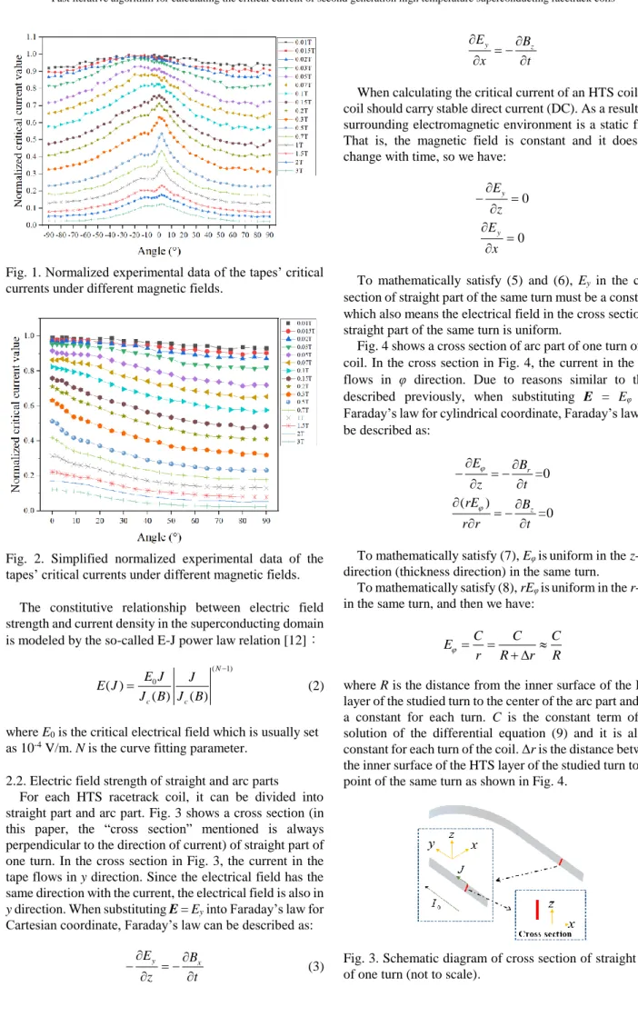
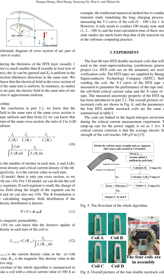
(2) Fast iterative algorithm for calculating the critical current of second generation high temperature superconducting racetrack coils. E y x. . Bz t. (4). When calculating the critical current of an HTS coil, the coil should carry stable direct current (DC). As a result, the surrounding electromagnetic environment is a static field. That is, the magnetic field is constant and it does not change with time, so we have: . E y. z E y. x. Fig. 1. Normalized experimental data of the tapes’ critical currents under different magnetic fields.. 0. 0. E. Br =0 z t  ( rE ) B   z =0 r r t. The constitutive relationship between electric field strength and current density in the superconducting domain is modeled by the so-called E-J power law relation [12]： EJ J E(J )  0 J c ( B) J c ( B). (2). 2.2. Electric field strength of straight and arc parts For each HTS racetrack coil, it can be divided into straight part and arc part. Fig. 3 shows a cross section (in this paper, the “cross section” mentioned is always perpendicular to the direction of current) of straight part of one turn. In the cross section in Fig. 3, the current in the tape flows in y direction. Since the electrical field has the same direction with the current, the electrical field is also in y direction. When substituting E = Ey into Faraday’s law for Cartesian coordinate, Faraday’s law can be described as: E y z. . Bx t. . (7) (8). To mathematically satisfy (7), Eφ is uniform in the z-axis direction (thickness direction) in the same turn. To mathematically satisfy (8), rEφ is uniform in the r-axis in the same turn, and then we have:. E . C C C   r R  r R. (9). ( N 1). where E0 is the critical electrical field which is usually set as 10-4 V/m. N is the curve fitting parameter.. . (6). To mathematically satisfy (5) and (6), Ey in the cross section of straight part of the same turn must be a constant, which also means the electrical field in the cross section of straight part of the same turn is uniform. Fig. 4 shows a cross section of arc part of one turn of the coil. In the cross section in Fig. 4, the current in the tape flows in φ direction. Due to reasons similar to those described previously, when substituting E = Eφ into Faraday’s law for cylindrical coordinate, Faraday’s law can be described as: . Fig. 2. Simplified normalized experimental data of the tapes’ critical currents under different magnetic fields.. (5). (3). where R is the distance from the inner surface of the HTS layer of the studied turn to the center of the arc part and it is a constant for each turn. C is the constant term of the solution of the differential equation (9) and it is also a constant for each turn of the coil. Δr is the distance between the inner surface of the HTS layer of the studied turn to any point of the same turn as shown in Fig. 4.. Fig. 3. Schematic diagram of cross section of straight part of one turn (not to scale)..

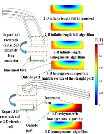
(3) Xiangyu Huang, Zhen Huang, Xiaoyong Xu, Wan Li, and Zhijian Jin. example, the traditional numerical method has to conduct a transient study simulating the long charging process of measuring the V-I curve of the coil (0 – 100 s for 1 A/s). However, it only needs to conduct 100 steady state studies (1, 2…100 A) and the total calculation time of these steady state studies are much faster than that of the transient study in the software computing practice. Fig. 4. Schematic diagram of cross section of arc part of one turn (not to scale). Considering the thickness of the HTS layer (usually 1 micrometer) is much smaller than R (usually at least tens of millimeters), the Δr can be ignored and Eφ is uniform in the r-axis direction (thickness direction) in the same turn. We can now know that the electrical field in the cross section of arc part of the same turn is uniform. In summary, no matter straight or arc part, the electric field in the same turn of one cross section is approximate uniform. 2.3. Algorithm From the conclusion in part 2.2, we know that the electric field in the same turn of the same cross section is approximate uniform and then from (2) we can know that for each turn of the same cross section, the ratio of J to Jc(B) is also uniform:. J1 J2 = = J c ( B1 ) J c ( B2 ).  J ds i. J. c. . ( Bi )ds. =. Jn  J c ( Bn ). c. The four 86-turn HTS double racetrack coils that will be used in the semi-superconducting synchronous generator project (i.e. HTS coils are on the armature) are used as verification coils. The HTS tapes are supplied by Shanghai Superconductor Technology Company (SSTC). Before winding the coil, the V-I curve of the HTS tape was measured to guarantee the performance of the tape and get the self-field critical current value and the N value of the tape. The measured anisotropy property of the HTS tapes has been introduced in part 2.1. The overall pictures of the racetrack coils are shown in Fig. 6, and the parameters of the four HTS double racetrack coils are the same and summarized in table Ⅰ. The coils are bathed in the liquid nitrogen environment during the critical current measurement experiment. The ramp-up rate for the power supply is set as 1 A/s. The critical current criterion is that the average electric field strength of the coil reaches 100 μV/m [13].. (10). I0. J. 3. EXPERIMENT. ( Bi )ds. where n is the number of meshes in each turn, Ji and Jc(Bi) is the current density and critical current density of the ith mesh respectively. I0 is the current value in each turn. For 2-D model, there is only one cross section, so we can directly use (10). For 3-D model, we can divide the coil into many segments. If each segment is small, the change of the electric field along the length of the segment can be neglected and we can also use (10). The A-formulation is used for calculating magnetic field distribution if the current density distribution is known:.  A= J. Fig. 5. The flowchart of the whole algorithm.. (11). where μ is magnetic permeability. From (10) we can know that the iterative update of current density in each turn of the coil is:. J i ( n 1) =J c ( Bi  n ). I0. J. c. (12). ( Bi  n )ds. where Ji-(n+1) is the current density value in the (n+1)th iterative step, Bi-n is the magnetic flux density value in the nth iterative step. The flowchart of the whole algorithm is summarized in Fig. 5. Take a coil with a critical current value of 100 A as. Fig. 6. Overall pictures of the four double racetrack coils..

(4) Fast iterative algorithm for calculating the critical current of second generation high temperature superconducting racetrack coils. Parameter. Value. Tape Manufacturer Tape thickness Tape width Substrate material N Critical current (77 K, self-field) b k Bc Turns Inner / outer radius of the coil Straight length Total length of HTS tapes. YBCO SSTC 1 um 4 mm Hastelloy 28 205 A 1.05795 0.0605 0.1942 T 86 37 / 54.2 mm 244 mm 66 m. 4. RESULTS AND DISCUSSIONS 4.1. Comparison of results of experiment and the proposed algorithm Fig. 7 shows the estimation results of five kinds of numerical models and the experiment results of the four coils. The first item in the legend is the numerical transient (the process of the current value ramping up at 1 A/s just like the experiment is simulated) model based on the commonly used H-formulation, and it regards the racetrack coil as infinite length conductor. For infinite length conductor, it can be expressed by one cross section as shown in Fig. 3 and it is just 2-D model. “Full” means each conductor is drawn separately and no homogeneous method [14] is used. The second item is the 2-D infinite length conductor model using the proposed algorithm without the homogeneous method and each conductor is still drawn separately. The third item is the 2-D infinite length conductor model using the proposed algorithm with the homogeneous method. The fourth item regards the racetrack coil as circular coil ignoring the straight part. It can be expressed by one cross section as shown in Fig. 4. The fifth item is the 3-D model considering both arc part and straight part. The match of the first three models proves the validity of the homogeneous method and the proposed algorithm. The calculation time for them are 2 h 48 min 23 s , 5 min 16 s and 2 min 32 s, respectively, and the proposed algorithm is much faster than the traditional numerical method. The 2-D axisymmetric model tends to underestimate the critical current and the 2-D infinite length model tends to overestimate comparing to the 3-D model. That is because for a given current amplitude, the magnetic field in the innermost turn of a circular coil (can be expressed by 2-D axisymmetric model) is larger than that of its corresponding racetrack coil [15]. Larger magnetic field means lower critical current density and higher electric field strength. As can be seen from Fig. 8, all these models show similar distribution patterns. The innermost turn of both arc and straight parts is under the largest magnetic flux density magnitude among all turns. For each turn of the coil, the outside end part exposes to the largest magnetic flux. density magnitude along the width direction of the YBCO tape. The average magnetic flux density magnitude in the arc part is larger than that in the straight part of the racetrack coil. The results of the 3-D model are more close to actual coils because only 3-D model can consider the interaction between straight and arc parts. The results of four experiment coils with the same geometric and tape parameters are different and such discrepancy can be caused by many reasons like the experimental measurement error and the non-uniformity of the tape along the length caused by the complicated HTS tape production process [16]. 2.0x10-4. Average electric field strength (V/m). TABLE Ⅰ COIL PARAMETERS.. 2-D infinite length full H transient 2-D infinite length full algorithm 2-D infinite length homogeneous algorithm 2-D axisymmetric homogeneous algorithm 3-D homogeneous algorithm Coil A Coil B Coil C Coil D. 1.0x10-4. 0.0 0 15 30 45 60 75 90. 94. 98. 102. 106. 110. 114. 118. 122. Current (A). Fig. 7. Comparison of V-I curve obtained by experiment and the proposed algorithm.. Fig. 8. Magnetic flux density magnitude distribution calculated by the proposed algorithm..

(5) Xiangyu Huang, Zhen Huang, Xiaoyong Xu, Wan Li, and Zhijian Jin. Fig. 9. The B-H curve of the studied silicon steel sheet.. Fig. 10. The relative position of the silicon steel sheet and the coil for each case.. 5.0x10-4. Average electric field strength (V/m). 4.2. Application: effect of the silicon steel sheet on the critical current of the racetrack coil In many actual applications like the HTS machine, the coil is placed along with the magnetic material. The existence of the magnetic material can divert the magnetic line [17], thus influencing the critical current value of the coil. Silicon steel sheet is a kind of commonly used magnetic material. The B-H curve of the studied silicon steel sheet is shown in Fig. 9 and it is also the material used in our group’s semi-superconducting synchronous generator project shown in Fig. 6. In this part, the iterative algorithm of the 3-D model is used for calculating the critical current under three silicon steel sheet layouts. The parameters of the studied coil are shown in Table Ⅰ, and each turn of the coil is numbered sequentially from the innermost turn to the outermost turn. As shown in Fig. 10, by comparing the results of case A with case B, C and D, the effect of the silicon steel sheet on the critical current of the racetrack coil can be qualitatively explained. We choose the turns numbered 1, 21 and 42, and calculate the critical current of them using the criterion of 100 μV/m to reflect the change in critical current value in 3 areas: inner, middle and outer of the coil.. A-1 A - 21 A - 42 B-1 B - 21 B - 42 C-1 C - 21 C - 42 D-1 D - 21 D - 42. 4.0x10-4. 3.0x10-4. 2.0x10-4. 1.0x10-4. 0.0 105. 107. 109. 111. 113. 115. 117. 119. 121. 123. 125. Current (A). Fig. 11. V-I curve of different cases obtained from the proposed algorithm. TABLE Ⅱ CRITICAL CURRENT OF EACH TURN. Turn number. Critical current (A). A-1 A - 21 A - 42 B-1 B - 21 B - 42 C-1 C - 21 C - 42 D-1 D - 21 D - 42. 112.8 114.5 122.1 105 (↓7.8) 113.3 (↓1.2) 120.7 (↓1.4) 113.5 (↑0.7) 116.6 (↑2.1) 118.8 (↓3.3) 114.3 (↑1.5) 113.3 (↓1.2) 110 (↓12.1). The V-I curves of different cases obtained from the proposed algorithm are shown in Fig. 11 and the critical current values are summarized in table Ⅱ (the values in parentheses are the critical current change values relative to case A). To understand the reason for the change in critical current value, the magnetic flux density magnitude distribution and magnetic lines of different cases calculated by the proposed algorithm are shown in Fig. 12. For case B, the inserted silicon steel sheet diverts magnetic field lines, gathering it to the silicon steel sheet faster. The vertical field component of the area near the silicon steel sheet increases relatively, and the critical current value of this area decreases. The innermost turn is most affected, and the critical current of it decreases more obviously. For case C, the silicon steel sheet above the coil attracts magnetic lines. For the first and 21th turn, the vertical field component drops slightly and the critical current values rises slightly, while the outermost turn is the opposite. For case D, the silicon steel sheet also attracts the magnetic lines, and the outermost turn is most affected. The vertical field component increases significantly and the critical current decreases significantly. However, the first and 21th turn relatively far away from the silicon steel sheet are less affected and the critical current values of them do not change much..

(6) Fast iterative algorithm for calculating the critical current of second generation high temperature superconducting racetrack coils. [2]. [3]. [4]. [5]. Fig. 12. Magnetic flux density magnitude distribution and magnetic lines of different cases calculated by the proposed algorithm (the current values are all 105 A and due to the symmetry, only one eighth of each model is displayed). In short, it can be found that the silicon steel sheet will increase the vertical field component of the HTS tapes close to it. Due to the anisotropy property of YBCO tapes, the critical current decay phenomenon is significant. However, the critical current change of the tapes far away from the silicon steel sheet is not obvious.. [6]. [7]. [8]. [9]. 5. CONCLUSION [10]. In this paper, a fast iterative algorithm for calculating the critical current of 2G HTS racetrack coils is introduced. It does not need to solve the long charging process which makes it faster than traditional transient numerical methods. The V-I curve of four 2G HTS double racetrack coils are measured verifying the validity of this algorithm. The effect of the silicon steel sheet on the critical current of the racetrack coil is also qualitatively studied. This algorithm could be used to design various large-scale applications employing 2G HTS racetrack coils efficiently.. ACKNOWLEDGMENT This work was supported by National Natural Science Foundation of China (Project No. 51707120) and Shanghai Marine Equipment Research Institute (Project No. 18H100000488).. [11]. [12]. [13]. [14]. [15]. [16]. [17]. REFERENCES [1]. Swarn S. Kalsi, Applications of high temperature superconductors to electric power equipment, John Wiley & Sons, 2011.. J. F. Maguire, et al., “Development and demonstration of a HTS power cable to operate in the long island power authority transmission grid,” IEEE Transactions on Applied Superconductivity, vol. 17, no. 2, pp. 2034-2037, 2007. Z. Huang, M. Zhang, W. Wang and T. A. Coombs, “Trial Test of a Bulk-Type Fully HTS Synchronous Motor,” IEEE Transactions on Applied Superconductivity, vol. 24, no. 3, pp. 1-5, 2014. Z. Hong, J. Sheng, J. Zhang, B. Lin, L. Ying, Y. Li, and Z. Jin, “The development and performance test of a 10 kV resistive typesuperconducting fault current limiter,” IEEE Transactions on Applied Superconductivity, vol. 22, no. 3, 2012. T. Konishi, T. Nakamura, T. Nishimura, and N. Amemiya, “Analytic evaluation of HTS induction motor for electric rolling stock,” IEEE Transactions on Applied Superconductivity, vol. 21, no. 3, pp. 1123-1126, 2011. Mark D. Ainslie, et al., “Simulating the in-field AC and DC performance of high-temperature superconducting coils,” IEEE Transactions on applied superconductivity, vol. 25, no. 3, pp. 1-5, 2014. D. Hu, et al., “DC characterization and 3D modelling of a triangular, epoxy-impregnated high temperature superconducting coil,” Superconductor Science and Technology, vol. 28, no. 6, p. 065011, 2015. Yingzhen Liu, et al., “Comparison of 2D simulation models to estimate the critical current of a coated superconducting coil,” Superconductor Science and Technology, vol. 32, no. 1, p. 014001, 2018. Rodriguez-Zermeno, Victor Manuel, et al., “Towards faster FEM simulation of thin film superconductors: A multiscale approach,” IEEE Transactions on Applied Superconductivity, vol. 21, no. 3, pp. 3273-3276, 2010. F. Grilli, F. Sirois, V. M. R. Zermeno, et al., “Self-consistent modeling of the Ic of HTS devices: How accurate do models really need to be?” IEEE Transactions on Applied Superconductivity, vol. 24, no. 6, pp. 1-8, 2014. F. Gömöry and B. Klinok, “Self-field critical current of a conductor with an elliptical cross-section,” Superconductor Science and Technology, vol. 19, no. 8, pp. 732–737, 2006. J. Rhyner, “Magnetic properties and AC-losses of superconductors with power law current—voltage characteristics,” Physica C: Superconductivity, vol. 212, no. 3-4, pp. 292-300, 1993. Min Zhang, et al., “Study of second generation, high-temperature superconducting coils: Determination of critical current,” Journal of Applied Physics, vol. 111, no. 8, p. 083902, 2012. Victor M. R. Zermeno, et al., “Calculation of alternating current losses in stacks and coils made of second generation high temperature superconducting tapes for large scale applications,” Journal of Applied Physics, vol. 114, no. 17, p. 173901, 2013. Víctor M. R. Zermeño and Grilli Francesco, “3D modeling and simulation of 2G HTS stacks and coils,” Superconductor Science and Technology, vol. 27, no. 4, p. 044025, 2014. K. Kubiczek, F. Grilli, A. Kario, A. Godfrin, V. M. R. Zermeno, M. Stępień, and M. Kampik, “Length Uniformity of the Angular Dependences of I c and n of Commercial REBCO Tapes with Artificial Pinning at 77 K,” IEEE Transactions on Applied Superconductivity, vol. 29, no. 1, pp. 1-9, 2018. Liu, Guole, Guomin Zhang, and Liwei Jing, "Experimental and numerical study of the frequency-dependent transport ac losses of the YBa2Cu3O7−δ coil with and without flux diverters,” Superconductor Science and Technology, vol. 32, no. 5 p. 055002, 2019..

(7)