Estimation of Rotation of Camera Direction and Distance Between Two Camera Positions by Using Fisheye Lens System

(1)

http://dx.doi.org/10.5369/JSST.2013.22.6.393 pISSN 1225-5475/eISSN 2093-7563

1. INTRODUCTION

Visual sensors have been widely used in various areas of computer vision to overcome several problems. One of these visual sensors is an omni-directional camera that provides a wide field of view of a scene that might cover almost a hemisphere or the entire 360° circle along the equator of a sphere. A fisheye lens is one of the most efficient ways to construct an omni-directional vision system [1-3]. Although fisheye lens cameras, which can be simply achieved by using a fisheye lens, provide us with the advantage of a wide angle of view, their images usually exhibit considerable distortion.

Several approaches have been reported to solve the behavior of fisheye lens images in the rotation and distance estimation for self-localization issues [2]. Self-localization is defined as the problem of finding the angle of rotation of a camera with respect to a reference direction and determining the distance of movement when a camera has moved from a certain reference position to a test position.

Zhao et al. proposed the use of calibration of the fisheye lens and analyzed the localization error parameters [4]. In calibrating the fisheye lens, their method included various parameters in order to reflect the characteristics of the fisheye lens system, thus introducing more computational complexity. Fu et al. proposed a landmark tracking with an embedded omni-directional vision system [5]. In their method, the navigator follows landmarks in order to localize the automatic guided vehicles. If the landmarks cannot be obtained, the localization is not successfully confirmed. Another method was proposed to estimate the distance of movement of a robot with a mounted omni- directional vision system with respect to the reference point in indoor environments that might possess natural color transitions by calculating the closest color transition in the environment [6]. However, in order for the system to work, a meaningful color transition should be observed in the environment, and its geometric map must be also known.

Xiong and Choi [7] proposed a self-localization method based on a fisheye lens and scale invariant feature transform (SIFT) [8] for indoor mobile robots. They discussed key point extraction, non-ceiling point removal, and keypoint calibration, but they did not provide the estimated distance and rotation of the mobile robot.

In this paper, we propose methods of estimating the rotation and the distance of a camera by using a fisheye lens system. First, we estimate the possible rotation of the camera direction at the new position because the correction of rotation is preferable during feature point matching at a

Estimation of Rotation of Camera Direction and Distance Between Two Camera Positions by Using Fisheye Lens System

Tewodros A. Aregawi

¹

, Oh-Yeol Kwon

¹

, Soon-Yong Park

²

, and Sung-Il Chien

^1,+

Abstract

We propose a method of sensing the rotation and distance of a camera by using a fisheye lens system as a vision sensor. We estimate the rotation angle of a camera with a modified correlation method by clipping similar regions to avoid symmetry problems and suppressing highlight areas. In order to eliminate the rectification process of the distorted points of a fisheye lens image, we introduce an offline process using the normalized focal length, which does not require the image sensor size. We also formulate an equation for calculating the distance of a camera movement by matching the feature points of the test image with those of the reference image.

Keywords : Vision sensor, Fisheye lens, Distance estimation, Rotation estimation

1

School of Electronics Engineering, Kyungpook National University, 80 Daehakro, Bukgu, Daegu, 702-701 Korea

2

School of Computer science and Engineering, Kyungpook National University, 80 Daehakro, Bukgu, Daegu, 702-701 Korea

+

Corresponding author: [email protected] (Received : Aug. 26, 2013, Accepted : Nov. 1, 2013)

This is an Open Access article distributed under the terms of the Creative Commons

Attribution Non-Commercial License(http://creativecommons.org/licenses/by-

nc/3.0)which permits unrestricted non-commercial use, distribution, and

reproduction in any medium, provided the original work is properly cited.

(2)

later stage. We estimate the rotation angle of the camera with a correlation method by clipping similar regions and suppressing the highlight areas of the images. The next step is to estimate the distance of the camera movement from the reference position to the new position called a test position. Image distortions occurring due to the nature of a fisheye lens require a complicated calibrating or rectifying method [4], but in our case, the concept of the normalized focal length, which is simply measured in an offline experiment, is introduced to avoid such rectification.

Salient points or feature points are defined and matched between two images, as we have developed an equation for finding the distance on the basis of a pair of matched points. For minimizing the error in distance estimation, these feature points should be quite stable and are obtained using the SIFT, which was also used elsewhere along with the Harris corner [8].

Section 2 presents the rotation estimation to find the direction of a camera, and Section 3 discusses the formulation of the distance estimation equation based on a normalized focal length and matching feature points.

Section 4 provides the experimental setup and results of our rotation and distance estimation. Section 5 concludes our work.

2. ROTATION ESTIMATION

In this section, we discuss a method for determining the rotation angle of a camera with respect to a reference position by using a correlation method. Further, we propose a method to overcome the problems in correlation, such as symmetry, and highlight areas to improve the accuracy of the angle estimation.

A camera can be placed in any direction with respect to its original orientation at the reference position. In this case, the camera captures images at the reference position as well as its new position, called a test position. Thus, we determine the angle of rotation of the camera by using these two images with a correlation method. The correlation method is used to compare the similarity of the two signals, resulting in a signal that shows the similarity between them and reaches its maximum when the two signals match best. Therefore, the maximum peak of the correlation of the two images corresponds to the estimated angle of the camera.

However, the image and its rotated image might look

similar, especially when the image contents are symmetric with respect to a rotation point or the center of the image in our case. Furthermore, highlights might appear inside an image area due to the lighting conditions of the environment. These two cases reduce the accuracy in estimating a rotation angle. Therefore, to solve the symmetry problem we remove a small portion of the central region of the image with careful radius selection. In addition, the highlight area detected with the help of Otsu’s thresholding method [9] is reduced in the grey level, leading to a reduction of its influence in the correlation.

The angle of rotation tells us how many degrees an image has rotated with respect to the original direction at the reference position. Now, we can re-rotate the rotated image by the estimated angle so that the camera direction of the test image is aligned with that of the reference image. This step is important for the distance estimation stage.

3. DISTANCE ESTIMATION

The overall distance estimation procedure for a camera moved from a reference position is presented in this section. We first explain a method of determining the normalized focal length of fisheye lens system to remove the rectification process of the distorted regions. Then, we develop a distance estimation formula by using the normalized focal length and a pair of matching feature points of two images. Finally, we discuss the selection of stable matching feature points to be utilized in the distance estimation.

3.1 Determination of the normalized focal length of the fisheye lens

It is known that fisheye lens images suffer from geometric distortion. The distortions in a fisheye lens can be explained when we observe the distance between two points in an image scene. The same distance within one image becomes bigger when the two points are projected around the center of the image than when projected around the boundary. Therefore, in order to deal with the distortion of the pixels, we introduce the concept of the normalized focal length for the fisheye lens system.

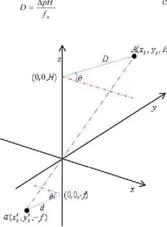
For this, we derive a relationship of the distance between

(3)

two positions of the camera in the real world and the displacement of the pixels in the corresponding image plane. We have illustrated this situation in Fig. 1, showing that when the camera travels a distance D, the pixels in the image plane move a distance d from the center. H denotes the height from the camera to the ceiling of the environment, and f represents the focal length of the fisheye lens camera, which is variable depending on its position from the center of the image. If the distance d in the image plane is divided by the pixel size of the complementary metal oxide semiconductor (CMOS) sensor, we can convert it to the corresponding pixel value denoted as p. Therefore,

where μ

s

is the pixel size of the camera sensor, and d is the corresponding actual distance traveled on the image plane.

On the basis of the relationship between the camera’s moved distance and the shift of the corresponding pixels in the image plane, as shown in Fig. 1, we have:

where f

n

is now called the normalized focal length of the fisheye lens camera. From Equation (3), we can deduce that even though the pixel size of the CMOS sensor is not provided, if we can measure p and D, we can obtain the normalized focal length, f

n

. This f

n

is required at the stage of distance estimation of a camera movement, but it varies depending on the pixel position (p) of a fisheye image. So it is necessary to obtain a lookup table for f

n

versus p.

For this, we place an object on the ceiling as a marker pointing to the center of the camera sensor. The camera is moved in a horizontal direction relative to the marking object capturing images at an interval of 25 cm for a total of 600 cm. The height, H, is set to 140 cm. Besides, the movement of the pixels (p) in the image plane at each interval can be registered. We can observe from Fig. 2 that the normalized focal length drops as the marker object moves from the center of the image to the outer boundary.

3.2 Distance estimation formula

A camera can move in any arbitrary direction in the xy- plane from a reference position to another test position. To figure out this situation, we have devised a model that calculates the actual distance moved by the camera and the displacement of image points in the image plane. In Fig. 3, the camera sensor points along the z-axis. Then, the original scene point at (0,0,H) moves to point A(x

S

,y

S

,H) by a distance D, whereas its corresponding image point moves from point (0,0,-f ) to point a(x

′_S

,y

′_S

,-f ) by a distance (1)

(2)

(3)

Fig. 1. An image model for estimating variable focal length of fisheye lens.

Fig. 2. Graph of normalized focal length versus pixel movement from center.

(4)

d or p in pixels in the image plane. In the corresponding image plane, we see that image point a is located at z = -f . Therefore, in the image plane, the arbitrary movement of the camera is described in terms of point a and f , which is the focal length of the fisheye lens camera.

For a camera that arbitrarily changes its position from a reference position, Equation (2) still holds true; so, we can estimate D from that equation. However, in this case, due to the arbitrary position of the camera, D is . The corresponding point movement in the image plane is given as

where d is the actual distance the camera has moved in the image plane, as in Equation (1). If d is divided by the camera CMOS size μ

s

, we can obtain p in Equation (1).

With this, we can assume one pair of matching feature points, one from the reference image (p

₁

) and the other from the test image (p

₂

). From these two points, we determine D as

where p = |p

1

_ p

₂

|, and f

n

=(– f

_n1

+f

_n2

)/2, in which f

_n1

and are the normalized focal lengths corresponding to p

¹

and p

2

; – f

n

is therefore their average.

In order to estimate D, f

n

must be given in advance when the pixel p is obtained in the test image. This step, therefore, requires the lookup table obtained from the graph of Fig. 2. We can think of an interpolation equation for the two variables, p and f

n

. However, we use the nearest neighbor method for simplicity, i.e., if p is given, we find the nearest p to the intervals in the graph and obtain the corresponding f

n

. This is because f

n

changes very slightly for most values of p.

3.3 Matching of feature points

An image has been first captured using a fisheye lens at the reference position. Then, the camera has been moved by some distance, and its direction might also be rotated. A new image has also been captured at the new position. At first, the image is re-rotated if a rotation has occurred. The next task is to match the feature points from the new image to the feature points from the original image at the reference position. Once the feature points are successfully matched between the two images, a pair of matching points is used to find the distance of a camera movement, which will be detailed later. For effective matching, we adopted the SIFT algorithm [8], which can provide stable and robust feature points. This algorithm has been well-studied and widely used, and thus its detailed description is omitted here. Among the detected feature points, the feature points with higher magnitudes are regarded as stable ones and selected as candidate points.

From the reference image, we extract a set of candidate feature points by using SIFT algorithm and we can represent their coordinates as (x

ⁱr

,y

ⁱr

), where i = 1, 2,..., N. N is the maximum number of extracted feature points from the image. For a test image, we extract a set of candidate feature points with coordinates (x

tⁱ

,y

ⁱt

) after its rotation correction. The next step is to perform matching among the set of candidate points of both images. The minimum Euclidean distance is used to match the points (x

ⁱr

,y

ⁱr

) and (x

ⁱt

,y

ⁱt

). Then, we obtain many combinations of matching feature points, but some points are wrongly matched. In order to discard the wrong matches and enhance the matching accuracy, we accept the matching feature points with higher magnitudes and select only 40 of all the points. Fig. 4 shows matching results for all the (4)

(5)

Fig. 3. Camera movement model in real world and image plane.

(5)

feature points and the selected 40 points based on their magnitude.

It is found that most of the 40 pairs of selected points are correctly matched, but sometimes wrong matching can occur, as indicated by the solid white line in Fig. 4(b). Most of the 40 matching feature points have a similar tendency in their direction. However, the lines between the wrongly matched points, such as the solid white line in Fig. 4(b), deviate from those of the correctly matched ones.

The distances from the 40 matching pairs are simply averaged as an estimated distance. Yet points that are located either around the center or the outer rims of the images tend to produce wrong matching, resulting in smaller or larger distances. Our analysis on the databases reveals that points producing smaller or larger distances should be removed from the estimation process. We found that the distances between some wrong matching pairs are usually less than the average, and we set this average value as the lower threshold. In order to remove large distances that are also prone to wrong matching, we first calculate the standard deviation (σ) as well as the average (μ) of these matching points. An experimental analysis suggests that the upper threshold is determined as μ+ 2.5σ. Thus, only the distances between the lower and upper thresholds are accepted and then averaged to obtain a final estimated distance.

4. EXPERIMENTAL RESULTS

4.1 Experimental setup

In order to obtain the images for the experiment, we use a fisheye lens on a Microsoft LifeCam camera with a resolution of 640×480. The images are taken at two different indoor environments. The first set of images has been taken in a room consisting of many shelves and different objects with lights on the ceiling, constituting the first image database (database 1). The second environment is a corridor inside a building that contains a small variety of objects such as the doors or windows of side rooms and lighting, of which the images constitute the second database (database 2).

Fig. 5 describes the positions at which each image is taken for each database. The camera reference position is located at the center of the coordinates. The experimental space is sampled into eight partitions, each represented by a line that is sampled at fixed intervals, as shown in Fig. 5.

Each black rectangle is the position of the camera. At each camera position, the camera rotates to eight directions at an interval of 45° with respect to the original camera direction.

Thus, the reference image is taken at the reference position, and a test image is taken eight times at a camera position denoted by the black rectangle. The camera positions have a 20 cm interval for a total of 100 cm; thus, we have 320 images for each database. Sample images for each database are shown in Fig. 6. The first row shows images from database 1, and the images in the second row are sample images of database 2.

Fig. 4. (a) Matching feature points for reference and test images with SIFT algorithm and (b) the 40 matching feature points that are selected.

Fig. 5. Diagram showing camera positions (small black rectangles)

and rotations at each camera position. At each camera

position, there are eight camera directions (one example is

shown inside the ellipse in the left side of the image).

(6)

4.2 Results of rotation and distance estimation Here, we will show the results of rotation estimation for the two databases. The results of both databases are quite similar, and thus, averaging has been performed over the two databases. The average values of the rotation estimation are given in Table 1. The first column indicates the actual rotation angle of the camera with respect to the reference position. The other column entries show the estimated rotation angle at a certain camera position (shown in the second row). Once a distance is chosen, we can find eight corresponding camera positions, and we calculate an average for a specific camera angle over those eight positions.

Now, we provide the average absolute rotation error in Table 2 to show the difference between the actual and estimated rotation angle. From Table 2, when the distance of the movement is up to 80 cm, the maximum average absolute rotation error is less than or equal to 4.24° with a relative error of 5.1%. In addition, we observe that the average absolute angle error tends to increase from short (20 cm) to long distances (100 cm). From this, we conclude that the accuracy in the rotation angle estimation of a camera at distances farther than 80 cm is not guaranteed by our method in our case.

Next, we discuss the distance estimation of camera movement. Table 3 shows the estimated distance moved by the camera at a specific camera position for the sample partitions. In Fig. 5, we can find the eight directions partitioning the space at an interval of 45 ^º . Each entry in

Fig. 6. Sample database images: (a) Reference image for database 1, (b) its test image (rotated 225° and moved 40 cm), (c) reference image for database 2, (d) its test image (rotated 225° and moved 40 cm).

Table 1. Average rotation angle estimation Actual

rotation angle(。)

Distance (cm)

0 -0.6 0.1 -0.4 2.6 11.4

45 43.1 42.3 41.0 39.6 33.9

90 88.2 88.2 85.6 85.1 73.7

135 129.9 131.3 131.7 130.4 137.8 180 178.9 176.9 176.3 177.2 151.0 225 222.2 228.4 221.3 219.3 212.4 270 267.8 266.1 265.4 266.9 267.8 315 316.1 316.9 316.1 314.9 303.3

20 40 60 80 100

Table 2. Average absolute rotation angle error Actual

rotation angle(。)

Distance (cm)

0 0.6 0.1 0.4 2.6 11.4

45 1.9 2.7 4.0 5.4 11.1

90 1.8 1.8 4.4 4.9 11.1

135 5.1 3.7 3.3 4.6 16.3

180 1.4 3.1 3.7 4.8 18.1

225 2.8 3.4 3.7 5.7 29.0

270 2.8 3.9 4.6 3.1 12.6

315 1.1 1.9 1.6 2.8 20.6

Average 2.2 2.7 3.2 4.2 17.5

20 40 60 80 100

Table 3. Average distance estimation

Direction (。)

Camera movement (cm)

0 19.7 42.2 58.1 75.9 84.3

45 18.6 37.8 59.6 76.3 84.2

90 22.0 37.4 56.1 78.9 85.8

135 19.7 39.5 56.6 72.7 87.9

180 17.7 42.3 56.5 74.8 80.9

225 19.7 39.3 53.4 72.7 82.2

270 20.1 40.0 55.6 72.2 85.1

315 20.2 39.9 56.6 74.6 82.0

Average 19.7 39.8 56.6 74.7 84.2

20 40 60 80 100

(7)

Table 3 is averaged over eight camera directions and two databases.

When the camera moves farthest (100 cm) from the reference position, the common matching area of the reference and test images shrinks down, thus reducing the accuracy in estimating the distance. The trade-off relation between the accuracy of distance estimation and the amount of camera movement is more clearly clarified in Table 4.

5. CONCLUSIONS

In this paper, we propose rotation and distance estimation methods for self-localization of a camera by using a fisheye lens system as a vision sensor. We have estimated the angle of rotation with a correlation method, and we remove similar regions that cause symmetry problems and suppress highlight areas for reliable results.

We use the fisheye lens to gain the advantage of a wide field of view. In order to remove the rectification process of the distorted points in a fisheye lens image, we devise a concept of normalized focal length of the fisheye lens. The distance estimation equation considers a pair of matched feature points from two images. The stable feature points are obtained from the SIFT feature space and are matched by using the minimum Euclidean distance. Our results confirm that the rotation and distance estimation methods can be applied to mobile robot applications such as self- localization and navigation.

ACKNOWLEDGMENT

This project was supported by the Civil Military Technology Cooperation Center and Korea Atomic Energy Research Institute.

REFERENCES

[1] Z. Cao, S. Liu, and J. Roning, “Omni-directional vision localization based on particle filter”, Image and Graphics ICIG, pp. 478-183, Sichuan, China, 2007.

[2] O. G. Bonin-Font, A. Ortiz, and G. Oliver, “Visual navigation for mobile robots: a survey”, Journal of Intelligent and Robotic Systems, Vol. 53, No. 3, pp.

263-296, 2008.

[3] N. Winters, J. Gaspar, G. Lacey, and J. Santos-Victor,

“Omni-directional vision for robot navigation”, IEEE Workshop on Omni-Directional Vision Proceedings, pp. 21-28, Hilton Head Island, USA, 2000.

[4] S. Zhao, B. Zhang, L. Li, and Z. Cao, “Fisheye lens camera system calibration and localization error analysis”, ICCDA, International Conference on Computer Design and Applications, pp. 441-445, Qinhuangdao, China, 2010.

[5] H. Fu, Z. Cao, and R. Juha, “Beacon tracking with an embedded omni-vision system”, International Conference of Natural Computation, pp. 274-278, Tianjin, China, 2009.

[6] M. Emanuele, P. Alberto, S. Alberto, and P. Enrico,

“Omni-directional vision scan matching for robot localization in dynamic environments”, IEEE Transactions on Robotics, Vol. 22, No. 3, pp. 523-535, 2006.

[7] X. Xiong and B. J. Choi, “Relative self-localization based on fish-eye lenses and SIFT algorithm for indoor mobile robot:”, Information Security and Assurance Communication in Computer and Information Science, pp. 389-394, Brno, Czech Republic, 2011.

[8] D. G. Lowe, “Distinctive image features from scale- invariant keypoints”, International Journal of Computer Vision, Vol. 60, No. 2, pp. 91-110, 1988.