Vol. 15, No. 11 pp. 6565-6575, 2014
Marginal Propensity to Consume with Economic Shocks - FIML Markov-Switching Model Analysis
Jae-Ho Yoon
1and Joo-Hyung Lee
2*1Senior Economist, POSCO Research Institute
2Graduate School of Urban Studies, Hanyang University
경제충격 시기의 한계소비성향 분석 - FIML 마코프-스위칭 모형 이용
윤재호1, 이주형2*
1포스코경영연구소, 2한양대학교 도시대학원
Abstract Hamilton's Markov-switching model [5] was extended to the simultaneous equations model. A framework for an instrumental variable interpretation of full information maximum likelihood (FIML) by Hausman [4] can be used to deal with the problem of simultaneous equations based on the Hamilton filter [5]. A comparison of the proposed FIML Markov-switching model with the LIML Markov-switching models [1,2,3] revealed the LIML Markov-switching models to be a special case of the proposed FIML Markov-switching model, where all but the first equation were just identified. Moreover, the proposed Markov-switching model is a general form in simultaneous equations and covers a broad class of models that could not be handled previously. Excess sensitivity of marginal propensity to consume with big shocks, such as housing bubble bursts in 2008, can be determined by applying the proposed model to Campbell and Mankiw's consumption function [6], and allowing for the possibility of structural breaks in the sensitivity of consumption growth to income growth.
요 약 본 논문에서 Hamilton의 마코프-스위칭 모형을 연립방정식으로 확장한 FIML 마코프-스위칭 모형을 제시해 보았다.
본 논문의 FIML 마코프-스위칭 모형을 LIML 마코프-스위칭 모형 등과 비교하면 LIML 마코프-스위칭 모형은 FIML 마코 프-스위칭 모형의 특별한 경우이며 FIML 마코프-스위칭 모형은 연립방정식으로 확장된 일반화된 모형 형태를 띄게 된다.
본 논문의 FIML 마코프-스위칭 모형을 Campbell and Mankiw 소비함수에 적용해 본 결과, 2008년 부동산 거품 붕괴와 같은 경제충격 시기의 한계소비성향은 매우 민감도가 높아진다는 것을 알 수 있다.
Key Words : FIML, LIML, instrumental variable, simultaneous equation, Markov switching, Hamilton filter, consumption, income, bubble burst
We are grateful to James D. Hamilton for his comments and suggestions. We are also grateful to Ronald Schoenberg and Chang-Jin Kim for putting their Gauss codes in the Internet Site.
*Corresponding Author : Joo-Hyung Lee(Hanyang Univ.) Tel: +82-2-2220-0276 email: [email protected]
Received September 30, 2014 Revised October 24, 2014 Accepted November 6, 2014
1. Introduction
This paper deals with an important issue associated with a class of the Markov-switching model in the simultaneous equations.
LIML(Limited Information Maximum Likelihood) Markov-switching models[1-3] estimate the parameters of a single equation. However, LIML models can be considered as a special case of the FIML(Full Information Maximum Likelihood) model where all but
⋯
⋯
⋮ ⋮ ⋱ ⋮
⋯
⋮
⋯
⋯
⋮ ⋮ ⋱ ⋮
⋯
⋯
⋯
⋮ ⋮ ⋱ ⋮
⋯
⋮
⋯
⋯
⋮ ⋮ ⋱ ⋮
⋯
⋯
⋯
⋮ ⋮ ⋱ ⋮
⋯
′
⋮
⋯
⋯
⋯
⋮ ⋮ ⋱ ⋮
⋯
⊗
⋯ the first equation are just identified.
This paper extends LIML Markov-switching models to a full set of structural simultaneous equations, essentially going from LIML to FIML with the addition to Markov-switching.
Using a framework for an instrumental variable interpretation of full information maximum likelihood by Hausman[4], this paper provides FIML Markov-switching model in the simultaneous equations.
The findings of this paper are that the proposed FIML Markov-switching model is a general form in the simultaneous equations and covers a broad class of models that could not be handled before. The advantage of the proposed FIML Markov-switching model is that we can deal with the problem of simultaneous equations based on the Hamilton filter[5]
and we can directly interpret the economic meaning of the estimated parameters without transformation of the model and the proposed FIML Markov-switching model don’t need another step to correct for the standard errors of the parameter estimates such as Kim’s LIML Markov-switching model[2].
In this paper the Campbell-Mankiw consumption on income problem[6] is used as an illustration.
This paper has been divided into five sections.
Section 2 presents the model specification. Section 3 compares the proposed FIML Markov-switching model to LIML Markov-switching models[1,3]. Section 4 summarizes the empirical results. Section 5 concludes this paper.
2. Model Specification
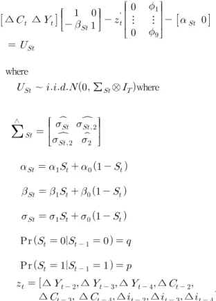
In order to get a consistent estimation of the parameters of the Markov-switching model in the simultaneous equations, we consider the following FIML Markov-switching model.
YBSt+ Z Γ St= U St,
U St∼i.i.d. N( 0,ΣSt⊗IT) (1)
where
Y is the T x M matrix of jointly dependent variables, BSt is an M x M matrix and nonsingular. Z is the T x K matrix of predetermined variables, ΓSt is
⋯
⋯
⋮ ⋮ ⋱ ⋮
⋯
K x M matrix positive definite and rank(Z) = K. USt is T x M matrix of the structural disturbances of the system. Thus, the model has M equations and T observations. The structural errors are assumed as a nonsingular M-variate normal (Gaussian) distribution.
σ is the covariance of the error terms. ∑St is a positive definite M by M matrix with no restrictions. It is assumed that all equations satisfy the rank condition for identification. Also if lagged endogenous variables are included as predetermined variables, the system is assumed to be stable. An orthogonality assumption, E(Z'USt)=0, between the predetermined variables and structural errors is required and, we assume the presence of contemporaneous correlation but no intertemporal correlation in (1). If we assume that the single Markov-switching variable St has an N-state, first-order Markov process, then we can write the transition probability matrix in the following way:
where pij= Pr (St= j |S t - 1= i) with
∑
Nj = 1pij= 1 for all i
To include different first order Markov-switching variables S1t, S2t, S3t,…, in the proposed model, we assume that the dynamics of an unobserved two-state, first order Markov-switching variables, S1t, S2t, S3t,…
are independent and can be represented by a single Markov-switching variable, St.
For example, if our model involves only two unobserved two-state first order Markov-switching variables such as S1t and S2t. The dynamics of Markov-switching variables such as S1t, S2t can be represented by a single Markov-switching variable St
in the following manner:
if
if
if
if with ,
Hausman[4] showed an instrumental variable interpretation of FIML for simultaneous equations where the function is maximized
·
′
·
′ (2)
where yt is the tth row of the Y matrix. zt is the tth row of the Z matrix.
To derive the FIML Markov-Switching Model in the simultaneous equations, we can obtain Pr (St= j| ψt) by applying a Hamilton filter[5] as follows:
Step 1 :
At the beginning of the tth iteration, Pr (St - 1= i |ψt - 1), i = 0,1,⋯,N is given.
And, we calculate
·
where ,
⋯, ⋯ are the transition probabilities.
Step 2 :
Consider the joint conditional density of yt and unobserved St= j variable, which is the product of the conditional and marginal densities:
from which the marginal density ofyt is obtained
where conditional density is obtained from (2):
·
′
(3) where
′
yt is the tth row of the Y matrix. zt is the tth row of the Z matrix. BSt and Γ
St is obtained from (1).
Step 3 :
Once yt is observed at the end of time t, we update the probability terms:
As a byproduct of the above filter in Step 2 we obtain the log likelihood function:
which can be maximized in respect to the parameters of the model.
3. Comparison of the proposed FIML MS model to LIML MS models
To solve the problems of the regressors being correlated with the disturbance in the Markov-switching models, we can adopt two models.
The first model is LIML Markov-switching model proposed by Kim[1,2] and Spagnolo, et al.[3]. The characteristics of LIML Markov-switching models
estimate the parameters of a single equation.
In the case of LIML Markov-switching model, the result of the “standard” estimation method proposed by Spagnolo, et al.[3] is mathematically identical to the
“alternative” estimation method proposed by Kim[1].
The second model is FIML Markov-switching model which we provide in this paper. The merit of the FIML Markov-switching model is that it provides the complete model in the case of simultaneous equations problem and solves the joint endogeneity of variables in simultaneous equations concurrently.
The gain of the reduction in the asymptotic covariance matrix in the FIML Markov-switching model brings with it an increased risk of inconsistent estimation. However, LIML Markov-switching models can be considered as special cases of the proposed FIML Markov-switching model where all but the first equation are just identified. Moreover, Kim’s LIML Markov-switching model[1,2] needs transformation of the model by Cholesky decomposition of the covariance matrix and Spagnolo, et al.[3] LIML Markov-switching model needs transformation of the model by 0 constraints on the covariance matrix of the residuals, whereas the proposed FIML Markov-switching model is a general model which does not need any transformation.
Spagnolo, et al.[3] LIML Markov-switching model is very similar to the example of Hausman[7] equation (2.3) which has 0 constraints on the covariance matrix of the residuals in the simultaneous equations.
When we compare the proposed FIML Markov-switching model to Kim’s LIML Markov-switching model[1], we find the proposed FIML Markov-switching model is mathematically identical to Kim’s LIML Markov-switching model[1]
with in equation (3). However, the difference between the proposed FIML model to Kim’s LIML Markov-switching model is that Kim’s LIML model needs another step to correct for the standard errors of the parameter estimates[2] but the proposed FIML model don’t need another step to correct for the
standard errors of the parameter estimates. Moreover, the proposed FIML Markov-switching model includes not only the case of , but also the case of
≠ .So Kim’s LIML Markov-switching model[1]
can be considered as a special case of the proposed FIML Markov-switching model.
4. Application
Let’s consider Campbell and Mankiw’s consumption model[6] as an example given by equations (4) and (5).
∆ ∆ (4)
∆ ′ (5)
where is the log of per-capita disposable income;
is the log of per-capita consumption on non-durable goods and services; and are correlated; ′ is a vector of instrumental variables not correlated with .
Following Campbell and Mankiw[6], the vector of instrumental variables employed ′ is given by
∆ ∆ ∆ ∆ ∆
∆ ∆ ∆ ∆
where is the first difference of the three-month T-bill rate. is interpreted as a fraction of aggregate income that accrues to individuals who consume their current income in the presence of liquidity constraints.
In equation (4) it can be seen that and ∆ are positively correlated, therefore would be overestimated by OLS. To solve the problem of the bias in the simultaneous equations (4) and (5), we can adapt the likelihood function of the simultaneous equations model in equation (2) following Hausman’s instrumental variable interpretation of FIM[4].
∆ ∆
′
⋮ ⋮
∧
While there seems to be a consensus that there isexcess sensitivity of consumption to current income which is represented by , there is a disagreement as to the source of this excess sensitivity and whether is constant or not.
In equation (4), Campbell and Mankiw[6] assume the constant .However, in light of the literature on precautionary saving, the parameter in equation (4) can also change when the economy is facing a great degree of uncertainty. Kimball[8] predicts that the marginal propensity to consume should have been higher in the 1970’s, when there was great uncertainty about the future rate of productivity growth. Kim[2]
adopts a two-step MLE procedure with a three-state Markov switching model using the same variables in Campbell and Mankiw[6] for quarterly real data from FRED, collected by the Federal Reserve Bank of St.
Louis. Kim[2] found that in th e 1970’s and 1980’s, during which time uncertainty in future income growth was highest, the measure of sensitivity was highest and statistically significant while it was not statistically significant in the rest of the sample.
Taking these into consideration in this paper, we try to find out whether is really constant or not. To do this, first we extend equations (4) and (5) in the following way which adopts simple two-state Markov switching parameters in order to incorporate structural breaks.
∆ ∆ (6)
∆ ′ (7)
where
∼
∆ ∆ ∆ ∆ ∆
∆ ∆ ∆ ∆
To solve the equations (6)-(7) together, we can rewrite them as follows:
where
∼ ∑⊗where
∆ ∆ ∆ ∆
∆ ∆ ∆ ∆ ∆
Fig. 1 depicts the relationship between Consumption
∆ and Income ∆
Fig. 2 depicts the two-state FIML Markov switching probabilities.
Fig. 3 depicts the two-state Kim's LIML Markov switching probabilities.
-4 -3 -2 -1 0 1 2 3 4 5
1960 1970 1980 1990 2000 2010
DINCOME DCONS
[Fig. 1] GDP ΔYt and Consumption ΔCt for U.S.
0.0 0.2 0.4 0.6 0.8 1.0
1960 1970 1980 1990 2000 2010
FIML USDATE
[Fig. 2] FIML Model : Probabilities of regime 1
0.0 0.2 0.4 0.6 0.8 1.0
1960 1970 1980 1990 2000 2010
KIM USDATE
[Fig. 3] Kim LIML Model : Probabilities of regime 1
0.0 0.2 0.4 0.6 0.8 1.0
1960 1970 1980 1990 2000 2010
FIML KIM
[Fig. 4] FIML vs Kim's LIML : Probabilities of regime
Parameters FIML Kim's LIML
1st OLS 2nd MLE
α0 0.23 (0.06)** 0.30 (0.05)**
α1 0.20 (0.06)* 0.23 (0.05)*
β0 0.47 (0.14)* 0.29 (0.09)*
β1 0.65 (0.11)** 0.57 (0.09)**
γ0 - -0.33 (0.09)*
γ1 - -0.26 (0.09)*
φ1 0.01 (0.04) 0.04 (0.07) - φ2 -0.09 (0.05) -0.11 (0.07) - φ3 -0.09 (0.05) -0.17 (0.07) - φ4 0.38 (0.11)* 0.21 (0.14) - φ5 0.62 (0.12)** 0.66 (0.15)** - φ6 0.06 (0.11) 0.28 (0.14) - φ7 -0.17 (0.06)* -0.25 (0.08)* - φ8 -0.03 (0.08) 0.08 (0.09) - φ9 -0.09 (0.06) -0.14 (0.08) -
σ0 0.24 (0.11) 0.21 (0.03)**
σ0,2 -0.37 (0.11)* -
σ1 0.24 (0.06)** 0.42 (0.03)**
σ1,2 -0.22 (0.08)* -
σ2 0.72 (0.07)** -
q 0.84 (0.14)** 0.89 (0.07)**
p 0.90 (0.10)** 0.95 (0.04)**
Log
Likelihood -402.68 -102.75
Standard errors are in the parentheses. *=significant at 5%
**=significant at 1%
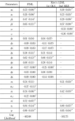
[Table 1] Maximum Likelihood Estimation (53Ⅱ∼14Ⅱ)
Table I reports estimation results for the proposed FIML Markov-switching model and LIML Markov-switching models.
The coefficients , of the FIML Markov-switching model are significant, and the degree of the upward movements is large, from 0.47 ( = ) to 0.65 ( = ).
The coefficients , of the FIML Markov-switching model are also significant. So, we can assume marginal propensity to consumption is not constant because the difference between and is large.
This result is same as the result of LIML Markov-switching models. The coefficients , of Kim’s LIML Markov-switching model are significant, and the degree of the upward movements is large, from 0.29 ( = ) to 0.57 ( = ). The coefficients
of Kim’s LIML Markov-switching model are also significant.
From the results of the FIML Markov-switching model and LIML Markov-switching models, we can conclude that marginal propensity to consumption is not constant.
From Figure 4, we can find that the inferred probabilities of the FIML and Kim's LIML Markov switching model are very similar to those of LIML Markov switching models.
However, the inferred probabilities
of the FIML Markov switching model and LIML Markov switching models accord with U.S recessionary dates after 1990. Especially we can find that a excess sensitivity of marginal propensity to consumption with big shocks such as housing bubble bursts in 2008.
We can also find that the inferred probabilities
are not consistent with Kimball[8], who suggests that the marginal propensity to consumption should have been higher in the 1970’s when there was great uncertainty about the future rate of productivity and income growth after two major OPEC oil shocks in 1973-1974 and 1979-1980.
5. Conclusion
In this paper, Hamilton’s(1989) Markov-switching model is extended to the simultaneous equations.
The proposed FIML Markov-switching model is applied to Campbell and Mankiw’s consumption function[6], by allowing for possibilities of structural breaks in the sensitivity of consumption growth to the income growth. From the empirical results of the FIML Markov-switching model and LIML Markov-switching models, we can conclude that marginal propensity to consumption is not constant. Especially we can also find that a excess sensitivity of marginal propensity to consume with big shocks such as housing bubble bursts in 2008.
Appendix I
I. COMPARISON OF KIM’S (2004) LIML MODEL TO THE SPAGNOLO, F., PSARADAKIS, Z. and SOLA M. (2005) LIML MODEL
1. THE SPECIAL CASE OF THE MARKOV- SWITCHING MODEL
In this section, we discuss representation of the special case of the Markov-switching model. Error terms are autocorrelated with AR(1). The model needs instrumental variables. The dynamics can be represented in the following manner:
(8) where
(9)
∼
≠ → ≠ → ≠ where is T x 1. The endogenous explanatory variable ⋯ is T x (M-1) and
is (M-1) x 1. The exogenous explanatory variable
⋯ is T x K1 and is K1 x 1.
is T x 1. is T x (M-1) and is (M-1) x (M-1). ⋯ is T x K2 and is K2x(M-1). We can consider and together as the instrumental variables in the equation (9) because of ≠ .
2. COMPARISON BETWEEN STANDARD AND ALTERNATIVE INSTRUMENTAL VARIABLE ESTIMATION
In equation (8) it can be seen that and are correlated. The procedure to derive a Markov-switching model is as follows:
(8)
(10)
After we calculate equation (8)-(10), we obtained the following Markov-switching model.
(11)
The standard instrumental variable estimation method proposed by Spagnolo, et al.[3]. needs the following two-step procedure.
Step 1: Regress on , and get from the equation (9).
Step 2: Insert to the eqs. (11) and get the following regression
(12)
The alternative instrumental variable estimation method proposed by Kim[1] needs the following two-step procedure.
Step 1: Regress on , and get residual
from the equation (9).
Step 2: Insert residual to the equation (11) and get the following regression
(13)
In order to show that equation (12) and (13) are mathematically identical, we need the following procedure from equation (12).
First, we get .
Second, insert to the equation (12), then we can get the following regression
(14)
The equation (14) is mathematically identical to the equation (13) with .
This result shows that the two estimation methods are mathematically identical even in the special case of the Markov-switching model.
Appendix II
1. COMPARISON OF THE PROPOSED FIML MODEL TO KIM’S LIML MODEL[1]
In order to show that Kim’s LIML Markov-switching model[1] is a special case of the
′
′
proposed FIML Markov-switching model, we canconsider the following Markov-switching model
(15)
(16)
In equation (15), is T x 1. The endogenous explanatory variable ⋯ is T x (M-1) and is (M-1) x 1. The exogenous explanatory variable ⋯ is T x K1 and is K1 x 1. The error term is T x 1. The reduced form of the equation in (16) has the instrumental variables and . is T x K1.
is K1 x (M-1). is T x K2, is K2x(M-1) and is T x (M-1). The covariance matrix of
∼ is given by (17).
′
(17)
where , ,
From equations (15) and (16), we obtain the likelihood function in the simultaneous equation
·
′
·
′ (18) where
,
,
,
,
,
,
“exptr” denotes “exponential and trace”
We can obtain by factoring as suggested by Radchenko et al.[9] as follows,
Then, the likelihood function in (18) may be transformed into
·
′
·
′
(19) where
′ ′ ,
, , and .
The equation (18) of the proposed FIML Markov-switching model is mathematically identical to the equation (19) of Kim’s LIML Markov-switching
m o d e l [ 1 ] with
≠ As Kim’s LIML Markov-switching model uses
′ instead of
. Kim’s LIML Markov-switching model needs another step to correct for the standard errors of the parameter estimates such as Kim[2] but the proposed FIML Markov-switching model don’t need another step to correct for the standard errors of the parameter estimates. Moreover, the proposed FIML Markov-switching model includes the case of in
equation. (18).
So, Kim’s LIML Markov-switching models can be considered as special cases of the proposed FIML Markov-switching model.
References
[1] C. J. Kim, "Markov-switching models with endogenous explanatory variables", Journal of Econometrics, 122, 1, pp.127-136, 2004.
DOI: http://dx.doi.org/10.1016/j.jeconom.2003.10.021 [2] C. J. Kim, "Markov-switching models with endogenous
explanatory variables II: A two-step MLE procedure with standard-error correction", Journal of Econometrics, 148, 1, pp.46-55, 2009.
DOI: http://dx.doi.org/10.1016/j.jeconom.2008.09.023 [3] F. Spagnolo, Z. Psaradakis, M. Sola, "Testing the Unbiased
Forward Exchange Rate Hypothesis Using a Markov Switching Model and Instrumental Variables", Journal of Applied Econometrics, 20, 3, pp.423-437, 2005.
DOI: http://dx.doi.org/10.1002/jae.773
[4] Jerry A. Hausman, "An instrumental variable approach to full information estimators for linear and certain nonlinear econometric models", Econometrica, 43, pp.727-738, 1975 DOI: http://dx.doi.org/10.2307/1913081
[5] J. D. Hamilton, "A new approach to the economic analysis of nonstationary time series and the business cycle", Econometrica, 57, 2, pp.357-384, 1989.
DOI: http://dx.doi.org/10.2307/1912559
[6] John Y. Campbell, N. Gregory Mankiw, "Consumption, Income, and Interest Rates: Reinterpreting the Time Series Evidence", In National Bureau of Economic Research Macroeconomics Annual 1989, eds. Oliver J.
Blanchard and Stanley Fisher, MIT Press, Cambridge MA, pp.185-216. 1989.
[7] Jerry A. Hausman, Whitney K. Newey, William E. Taylor,
"Efficient Estimation and Identification of Simultaneous Equation Models with Covariance Restrictions", Econometrica, 55, pp.849-874, 1987.
DOI: http://dx.doi.org/10.2307/1911032
[8] Miles S. Kimball, "Precautionary savings and the marginal propensity to consume", NBER Working Paper No. 3403, 1990.
[9] S, Radchenko, H. Tsurumi, "Limited Information Bayesian Analysis of a Simultaneous Equation with an Autocorrelated Error Term and its Application to the U.S.
Gasoline Market", Journal of Econometrics, 133, pp.31-49, 2006.
DOI: http://dx.doi.org/10.1016/j.jeconom.2005.03.008
Jae-Ho Yoon [Regular member]
•Aug. 1989 : Korea Univ., Dept.
of Economics, Bachelor
•Feb. 1994 : Korea Univ., Dept of Economics, Master
•Oct. 2014 : Hanyang Univ., Graduate School of Urban Studies, Ph.D. Candidate
•Nov. 1995 ∼ current : POSCO Research Institute, Senior Economist
<Research Interests>
Urban Development and Housing Policy, Urban Economics(North Korea), Supercomputer
Joo-Hyung Lee [Regular member]
•Feb. 1979 : Hanyang Univ., Architecture Engineering, Bachelor
•May 1983 : Cornell Univ., Urban Planning, Master
•Jun. 1985 : Cornell Univ., Urban Planning, Ph.D.
•Mar. 1986 ~ current : Hanyang Univ., Graduate School of Urban Studies, Professor
<Research Interests>
Urban Regeneration, Urban Culture, Urban Development and Housing Policy