Design of the Optimal Grinding Process Conditions Using Artificial Intelligent Algorithm

1. 서 론

일반적으로 연삭공정은 기계가공의 마지막 단계에서 이루 어지는 작업으로 공작물의 정밀도를 결정하는 중요한 공정 이다. 이러한 공작물의 정밀도와 가공 경비는 작업자의 숙련 도에 따라 많은 부분 영향을 받는다. 따라서 연삭공정을 통 한 가공물의 가공 상태를 예측하기 위해서 여러 연삭 프로

세스 모델 들이 개발되어왔다. 이 중 대표적인 연삭 프로세 스 모델은 거칠기, 파워(Power), 버닝(Burning) 모델 및 G-ratio등이 있다

^(1,2)

* 동아대학교 고기능성밸브기술지원 지역혁신센터 ([email protected]) 주소: 604-714 부산시 사하구 하단2동 840번지

인공지능 알고리즘을 이용한 최적 연삭 공정 설계

최정주*

(논문접수일 2009. 06. 29, 심사완료일 2009. 11. 12)

Design of the Optimal Grinding Process Conditions Using Artificial Intelligent Algorithm

Jeongju Choi*

Abstract

The final quality of the workpiece is affected by the grinding process that has been conducted in final manufacturing stage. However the quality-satisfaction of ground workpiece depends on the skill of an expert in this process. Therefore, the process models of grinding have been developed to predict the states according to grinding process. In this paper, in order to find the optimized grinding condition to reduce the manufacturing expense and to meet requirements of ground workpiece optimization algorithm using E.S.(Evolutionary Strategy) is proposed. The proposed algorithm has been employed to find the optimal grinding and dressing condition using the grinding process models and nonlinear grinding constraints. The optimized results also presents the guide line of grinding process. The effectiveness of the proposed algorithm is verified through the experimental results.

Key Words : 플런지연삭(Plunge grinding), 거칠기모델(Roughness model), 진화전략(Evolutionary strategy), 최적제어(Optimal control)

Table 1 Power models for plunge grinding wheel/

workpiece 파워 모델 식 Peters

⁽⁵⁾

100Cr6



_

_



_



^

^

_ ^

Li

⁽⁶⁾

steel(GCr15)



_





_



_

   

_



_



^

^{}

Xio

⁽⁷⁾

AISI52100



 _

_

 _

_

 _

 _



_

_



_



×

_

_

^  _

 _

 _

^

   × 

^{ }

_ ^

_ ^

Werner

(8)

Ck45N



_



 _

^

_



_



^{  }

^

_ ^{  }

Shin

⁽²⁾

4140 Rc40





_



_ ^



_

_

_ ^{ }

_ ^{ }

_ ^{ }

_ ^{ }

_

Table 2 Roughness models for plunge grinding wheel/

workpiece 거칠기 모델 식

Lindsay

(8,9)

2A80K4VF MB/

AISI52100

 _

_

 _ ^{ }



_ ^{ }

  

_



_



_ ^{ }



_ ^{ }



_

 _













_  _ ^

 _



_  _ ^

 _

Snoeys

(10)

100Cr6

 _

 _

_ ^{ }

Chiu

⁽¹¹⁾

AISI52100

 _

_

_ ^

_ ^

_ ^

_



_



×

_

_

_

Konig

(12)

EK80JotKe/

Riegger NSS 10710

 _

_

_ ^{ }  _ ^{′ }

 _ ^′

_

^{ }

 

_

_ ^{ }  _ ^{′ }

 _ ^′

_

^{ }

Chen

⁽¹³⁾

Si3N4

 _

_ ^



_

^

_



_

^⋅



Shin

⁽²⁾

4140 Rc55

 _

 _

 _∞

 _

  

^{   ′}

 _

_

_ ^{ }

_ ^{ }

_ ^{ }

^{    }

 _∞

_

_ ^{ }

^{    }

′

 최적의 연삭 조건을 선정하는 방법과 가공비용에 근거한

평가 함수를 이용하는 방법 등이 제안되었다

^(3,4)

^(2,3,14)

제안한 최적화 알고리즘은 실험적으로 규명한 연삭공정 모델과 연삭기의 하드웨어적인 한계 및 가공물의 버닝 조건 등이 고려될 수 있도록 설계하였다. 제안된 알고리즘의 검토 를 위하여 본 논문에서는 플런지(Plunge) 연삭에 대한 연삭 공정 모델 및 평가함수를 설계하고 시뮬레이션 및 실험을 수행하였다.

본 논문의 구성은 2장에서 거칠기 및 파워 모델을 포함한 연삭공정 모델식과 연삭공정 모델의 파라미터 규명을 위한 실험조건 및 결과를 나타냈었다. 그리고 최적 연삭 조건 선 정을 위한 평가 함수와 구속 조건을 3장에 기술하였다. 4장 에서는 E.S.를 이용한 최적 연삭 조건 선정 및 실험결과를 나타내었다. 끝으로 5장에서 결론을 기술하였다.

2. 최적 연삭 조건 선정을 위한 연삭공정 모델

연삭공정에 따른 공작물의 가공 상태를 나타내기 위한 연 삭공정 모델들은 앞선 연구자들에 의해 다양한 형태로 제안 되어 왔다. 대표적인 연삭공정 모델은 가공 파워와 거칠기 모델이 있다. 이 중 가공 파워 모델은 연삭숫돌과 공작물사 이의 수직하중 사이의 관계를 이용하여 표현할 수 있다. 이 때 작용하는 수직하중은 연삭숫돌의 드레싱 및 연삭 조건에 따라 차이를 나타낸다. 이러한 연삭 가공 파워 모델은 Table 1과 같이 공작물 및 연삭숫돌의 종류에 따라 여러 형태로 제안되어왔다.

Table 1에서 제시된 파워 모델들은 연삭공정이 진행됨에 따라 숫돌의 마모 또한 진행되어 연삭에 필요한 가공 파워는 선형적으로 증가함을 나타낸다.

Table 2는 연삭 가공에 따른 공작물의 표면 거칠기 변화 를 나타내는 거칠기 모델들을 정리하였다. 거칠기의 변화는 드레싱 조건에 영향을 받는 초기 거칠기와 연삭 조건에 영향 을 주로 받는 거칠기 모델식이 있다.

Table 3 Experimental conditions for the initial power model

Level 1 Level 2 Level 3

s d

u [mm/sec]

d w

a d

v s [mm/sec]

t s [sec]

Table 4 Experimental conditions for the initial roughness model

Level 1 Level 2 Level 3

s d

u [mm/sec]

t

s [sec]

a d

v s

d w [sec]

Table 5 Experimental conditions for initial models using D-optimal algorithm



_

_

_

1 Level 1 Level 2 Level 1 2 Level 1 Level 3 Level 3 3 Level 1 Level 1 Level 2 4 Level 1 Level 2 Level 2 5 Level 2 Level 2 Level 2 6 Level 2 Level 3 Level 1 7 Level 2 Level 1 Level 3 8 Level 2 Level 1 Level 3 9 Level 3 Level 2 Level 3 10 Level 3 Level 1 Level 1 11 Level 3 Level 3 Level 3 12 Level 3 Level 3 Level 2 Table 1과 2에서 제안된 파워 및 거칠기 모델 중 Shin에

의해 제안된 모델은 기존의 연삭공정 모델들에서 사용된 파 라미터들을 통계적 방법으로 분석하여 중요 파라미터를 정 하고 이를 바탕으로 모델을 개발하였다.

Shin에 의해 제안된 모델은 4140(HRC40, HRC55), 8620 (HRC40) 합금강과 32A-60-K-VBE와 94A-8-M-V18 연삭 숫돌을 이용하여 제안한 모델에 대한 검증을 하였다. 본 연 구에서는 Shin의 실험에서 사용한 연삭숫돌과 합금강을 사 용하여 모델 검증에 대한 실험을 생략하고 모델 파라미터 선정을 위한 실험만을 하였다.

다음으로 연삭 중 과도한 절입 속도에 의한 공작물의 버닝 상태를 예측하기 위한 버닝 모델은 Markin에 의해 실험적으 로 식 (1)과 같이 규명 하였다

⁽¹⁾

 ^

_

_ ^

^

_ ^

여기서 

_

_

다음은 연삭 작업 중 연삭숫돌의 누적 마모량에 대한 공작 물의 절삭량 비를 나타내는 G-ratio이다.



 _

_ ^{ }

 _



_



_



^{ }

여기서 

_

 _

_

_

이상의 연삭공정 모델에 대한 파라미터 추정을 위해 실험에 사용한 연삭기는 G20-50CNC이며 연삭 숫돌은 32A-60-K- VBE를 사용하였다. 그리고 실험에 사용된 시편은 지름 63.5[mm], 폭 19.54[mm]의 원통형으로 4140 alloy steel (RC40) 열처리 시편을 이용하였다. 초기 파워 및 거칠기 모델

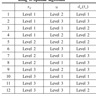
에 대한 파라미터추정 실험 조건은 Table 3과 4에 나타내었 다. 본 연구는 배치(batch)단위 연삭공정에서 연삭공정이 연 속적으로 이루어질 때 매회 수행되는 최적의 연삭조건 선정을 위한 알고리즘 개발에 그 목적이 있으므로 각 모델에 대한 파라미터 규명을 위한 실험은 D-optimal알고리즘을 이용하 여 최소의 실험회수를 수행하도록 하였다. Table 5는 두 모델 에 대한 D-optimal알고리즘으로 선정된 12번의 실험순서이다.

Fig. 1은 Table 3과 5의 연삭 조건에 근거하여 수행한 실험결 과이다. 실험의 결과에서 추정치는 Matlab ver.7.1의 비선형 커브피팅 함수를 이용하여 구하였다. 추정된 파워 모델은 식 (3)에 나타내었다.



_

_ ^{ }

_ ^{ }

_ ^{}

_ ^{}

_

Fig. 1 Specific power for the initial power model

Fig. 2 Roughness for the initial roughness model

Table 6 Experimetal conditions for power model

s d

u [mm/sec] t s

h eq

0.1283

0.00847

20

h eq

h eq

Table 7 Experimetal conditions for roughness model condition [unit]

h eq

h eq

u [mm/sec]

t s [sec]

a d [mm]

s d [mm/rev]

 _

_ ^{ }

_ ^{}

_ ^{}

^{  }

여기서 

_

_

_

_

_

 _

Fig. 2는 Table 4와 5의 조건을 바탕으로 수행한 초기 거 칠기 모델 규명을 위한 실험으로 드레싱 직후의 거칠기를 나타내는 결과이며 이에 대한 추정치는 식 (4)와 같다.

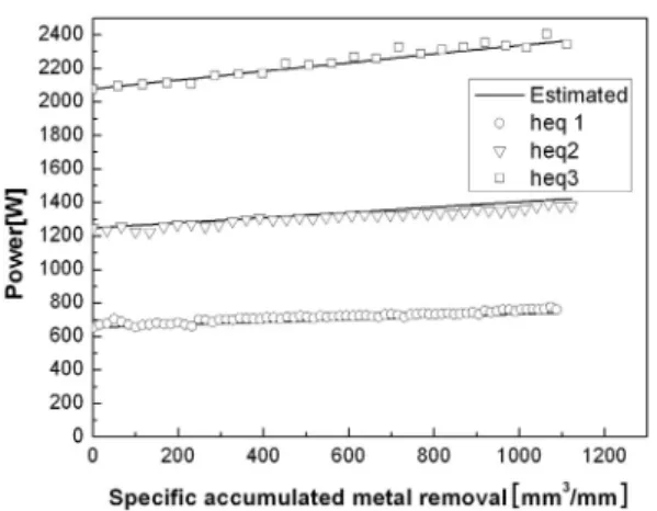
다음은 연속적인 연삭작업을 통해서 나타나는 가공 파워 와 거칠기 변화를 규명하기 위해서 실험조건을 Table 6과 7로 선정하였다. 이는 배치단위로 이루어지는 연삭작업에서 파워의 변화는 식 (3)과 (5)와 같이 초기 파워



_

속도(의 함수로 표현할 수 있으므로 Table 6과 같은 실험 조건을 선정하였다. 거칠기 변화 모델의 경우는 식 (6), (7) 과 같이 등가 칩두께(

_





_

^{ } 

_

 _∞

_ ^{}

^{  }

 _

 _

 _∞

 _

^{ ′ }

여기서



_



_

Table 7의 실험 조건에 근거한 실험결과는 Fig. 4에 나타 내었다. 추정된 모델식은 식 (6), (7)과 같다.

3. 최적 연삭 조건 선정을 위한 평가 함수 및 구속조건

연삭 작업의 최적 조건을 구하기 위해서 우선 다음과 같은 평가 함수를 선정하였다. 선정된 평가 함수는 각 사이클에 소요되는 연삭 비용과 드레싱 비용을 고려하였다.

 _

  



 _

 _

_

Fig. 3 Power against specific accumulated metal emoval

Fig. 4 Roughness against specific accumulated metal removal

 _

_



_

_

_

 _

_

 _



_

_

 

 _



_

_

 (9)

 _

 _

 _

(10)

여기서

 _

 _

_



_



_

_

 _

_

_

_

 _

 _

 _

 _

_

입력 변수이다.



_

_

_

_

_  _

_

_

여기서 

_

 _

_

_

황삭 및 정삭 가공 시간에 대한 구속조건은 다음의 관계를 가진다.



_

_



_

, 

_

_



_

 

_

  

_

(12)

여기서 은 최대 절삭 깊이 이다.

다음은 선정된 평가 함수의 최적값 선정에 있어 공작물에 버닝이 일어나지 않으면서 거칠기, 가공 파워 등의 요구 조 건에 대한 한계치이다.

(a) 절입속도에 대한 한계치



_ ^

_

_ ^

_ ^

_

_ ^

여기서 

_ ^

_ ^

_ ^



_ ^

(b) 버닝 연삭이 일어나지 않기 위한 가공파워 한계치



_

 ^

 ^

_

_ ^

^

_ ^

(c) G ratio의 한계치

 ^



 ^

(d) 가공파워 및 거칠기 한계치

 ^



 ^

 _ ^

 _

 _ ^

이상과 같이 선정한 가공 한계치는 Table 8에 정리하였다.

4. E.S. 알고리즘을 이용한 플런지 연삭 시스템의 최적화

E.S 알고리즘은 유전자 알고리즘의 한 분야로써 돌연변이

Table 8 Constraints for the grinding

연삭 조건 경계치 최소 최대

황삭 조건

Depth of cut [mm] 0.5 0.6 Infeed rate [mm/s] 0.01 0.04 Grinding Power [W] 0 2300 Grinding ratio 25 1000

정삭 조건

Depth of cut [mm] 0.05 0.2 Infeed rate [mm/s] 0.004 0.02 Grinding Power [W] 0 2300 Grinding ratio 25 1000

기타 조건

Spark out time 0 10 Roughness [

μ m]

No burning

Table 9 Optimized grinding conditions 드레싱 조건

Dressing depth [mm] 0.0594 Dressing lead [mm/rev] 0.1094

Dressing interval 6 황삭 조건

Depth of cut [mm] 0.6 Infeed rate [mm/s] 0.04 Roughing time [sec] 15

정삭 조건

Depth of cut [mm] 0.1 Infeed rate [mm/s] 0.02 Finishing time [sec] 5

기타

Spark out time [sec] 3.6 Wheel speed [rpm] 180 Workpiece speed [rpm] 2000

연삭 비용/사이클 [원] 371.46

전체 비용 [원] 2245.4

가 주된 조작이다. 이는 부모 벡터에 평균이 0인 정규분포 난수벡터를 가하는 방법으로 이루어진다.

주 연산은 재조합(Recombination)에 의해 이루어지며 보조연산으로 돌연변이(Mutation), 선택(Selection)의 연산 에 의해 최적의 해를 구하게 된다.

돌연변이는 하나의 개체 ()와 같이 탐색공간내의 위치 벡터와 표준편차 벡터의 쌍으로 구성되며 일반적으 로 돌연변이에 의한 다음 세대의 개체는 다음과 같이 나 타낸다.

′      

 _

^

′  

_

^{ }

여기서 ′ 는 자손(Offspring),   은 부모(Parents),

 _

^

이러한 연산은 다음의 알고리즘으로 동작한다.

procedure ES() initialize(Population);

evaluate(Population);

Parents = selection(Population)

while not (terminal condition satisfied) do MutationPool = recombination(Parents);

Offsprings = mutation(MutationPool);

evaluate(Offsprings);

Parents = selection(Offsprings);

end while end procedure

선정된 평가함수와 가공 한계치를 바탕으로 E.S. 알고리 즘을 적용하여 선정한 최적 연산 조건은 Table 9와 같다.

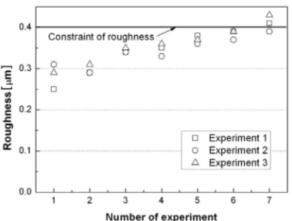
Table 9과 같이 추정된 최적 연삭 조건을 이용하여 실험 적으로 그 결과를 검증하였다. 검증을 위한 실험을 3차례에 걸쳐 수행하였고 그 결과를 Fig. 5에 나타내었다. 결과에서 E.S. 알고리즘을 통해 선정한 연삭 조건으로 수행한 연삭 작 업은 7번의 연삭 작업 이후 그 거칠기 한계인 0.4를 벗

Fig. 5 Roughness against specific accumulated metal removal

어났으나 한 번의 경우에 있어서는 거칠기 한계 이내에서 가공이 이루어 졌다.

5. 결 론

기계 가공의 마지막 단계에서 이루어지는 연삭 작업은 그 비용이 작업자의 숙련도에 따라 많은 부분 결정된다. 그 러나 연삭공정에 따른 공작물의 거칠기를 본 논문에서 제시 한 연삭공정 모델을 이용한 최적 연삭 조건 선정 알고리즘을 적용함으로써 그 가공 경비의 절감과 최적의 가공 조건을 선정 할 수 있다. 제안된 알고리즘의 검증을 위해 실시한 실 험의 결과에서 공작물의 거칠기는 요구 사양에 부합하였으 나, 일부의 경우에 있어서는 최적을 조건을 추정하지 못함을 알 수 있었다. 이러한 부분은 연삭 작업 의 복잡한 비 선형성 에 의한 것으로 사료된다. 그러나 제시된 알고리즘은 실제 큰 배치(batch) 단위의 연삭 작업에서 비 숙련자라 하더라도 최적의 기계가공을 위한 가이드라인으로 충분히 활용될 수 있을 것으로 사료된다.

후 기

본 연구는 지식경제부 지정 지역혁신센터사업(RIC) 고기 능성밸브기술지원센터 지원으로 수행되었음.

참 고 문 헌

(1) Markin, S., 2008, Grinding Technology: Theory and

Application of Machining with Abrasives, John Wiley

& Sons, New York.

(2) Choi, T. J., Subrahmanya, N. and Shin, Y. C, 2008,

“Generalized practical models of cylincrical plunge grinding proceses,” Machine Tools and Manufacture, Vol. 48, pp. 61~72.

(3) Xiao, S. and Markin, S, 1996, “On-line Optimization for Internal Plunge Grinding,” CIRP-Manufacturing

Technology, Vol. 45, No. 1, pp. 287~292.

(4) Xiao, G., Malkin, S. and Danai, K., 1993, “Automated system for multi-stage cylindrical grinding,” ASME

Journal of Dynamic Systems, Measurement, and Control, Vol. 115, pp. 667~672.

(5) Perters, J., Snoeyes, R. and Decneut, A., 1976, “The proper selection of grinding conditions in cylindrical plunge grinding,” Annals of the CIRP, Vol. 26, No.

1, pp. 387~394.

(6) Li, L. and Fu, J., 1980, “A study of grinding force mathematical model,” Annals of the CIRP, Vol. 29, No. 1, pp. 245~249.

(7) Xio, G., Malkin, S. and Danai, K., 1993, “Auto- mated system for multi-stage cylindrical grinding,”

ASME Journal of Dynamic Systems, Measurement and Control, Vol. 115, pp. 306~313.

(8) Werner, G., 1978, “Influence of work material on grinding forces,” Annals of the CIRP, Vol. 27, No.

1, pp. 243~248.

(9) Lindsay, R. P. and Hahn, S., 1973, “On the surface finish-metal removal relationship in precision grinding,”

Annals of the CIRP, Vol. 22, No. 1 pp. 105~106.

(10) Snoyes, R., Peters, J. and Decneut, A., 1974, “The significance of chip thickness in grinding,” Annals

of the CIRP, Vol.23, No. 2, pp. 227~237.

(11) Chiu, N. and Malkin, S., 1993, “Computer simulation for cylindrical plunge grinding,” X. M. Wen, A. A.

O. Tay, A. Y. C. Nee, 1992, “Micro-computer-based optimization of the surface grinding process,” Annals

of the CIRP, Vol. 42, No. 1, pp. 383~387.

(12) Konig, W. and Steffens, K., 1982, “A numerical method to describe the kinematics of grinding,”

Annals of the CIRP, Vol. 31, No. 1, pp. 201~206.

(13) Wen, X. M., Tay, A. A. O. and Nee, A. Y. C.,

1992, “Micro-computer-based optimization of the surface grinding process,” Annals of the CIRP, Vol.

42, No. 1, pp. 383~387.

(14) Yoo, S. M., 2008, “A Study on the Flexible Disk

Grinding Process Parameter Prediction Using Neural Network,” Transactions of the Korean Society of

Machine Tool Engineers, Vol. 17, No. 5, pp.

123~130.