• 검색 결과가 없습니다.

Univariate Analysis of Soil Moisture Time Series for a Hillslope Located in the KoFlux Gwangneung Supersite

N/A
N/A
Protected

Academic year: 2021

Share "Univariate Analysis of Soil Moisture Time Series for a Hillslope Located in the KoFlux Gwangneung Supersite"

Copied!
12
0
0

로드 중.... (전체 텍스트 보기)

전체 글

(1)

Univariate Analysis of Soil Moisture Time Series for a Hillslope Located in the KoFlux Gwangneung Supersite

Mina Son 1 , Sanghyun Kim 1 * , Dohoon Kim 1 , Dongho Lee 2 , and Joon Kim 2

1

Department of Environmental Engineering, Water resource and Environment Laboratory, Pusan National University, Busan, 609-735, Korea

2

Department of Atmospheric Sciences / Global Environment Laboratory, Yonsei University, Seoul, 120-749, Korea

(Received March 20, 2007; Accepted June 11, 2007)

광릉수목원 내 산지사면에서의 토양수분 시계열 자료의 단변량 분석

손미나 1 ·김상현 1 ·김도훈 1 ·이동호 2 ·김 준 2

1

부산대학교 환경공학과,

2

연세대학교 대기과학과/지구환경연구소 (2007년 3월 20일 접수; 2007년 6월 11일 수락)

ABSTRACT

Soil moisture is one of the essential components in determining surface hydrological processes such as infiltration, surface runoff as well as meteorological, ecological and water quality responses at watershed scale. This paper discusses soil moisture transfer processes measured at hillslope scale in the Gwangneung forest catchment to understand and provide the basis of stochastic structures of soil moisture variation.

Measured soil moisture series were modelled based upon the developed univariate model platform. The modeling consists of a series of procedures: pre-treatment of data, model structure investigation, selection of candidate models, parameter estimation and diagnostic checking. The spatial distribution of model is associated with topographic characteristics of the hillslope. The upslope area computed by the multiple flow direction algorithm and the local slope are found to be effective parameters to explain the distribution of the model structure. This study enables us to identify the key factors affecting the soil moisture distribution and to ultimately construct a realistic soil moisture map in a complex landscape such as the Gwangneung Supersite.

Key words : Soil moisture, Time series, Univariate analysis, ARMA model

I. INTRODUCTION

Soil moisture is an important intermediate hydrolog- ical variable because it determines infiltration, evapo- transpiration, solute transport, runoff generation and even hillslope scale ecosystem (Georgakakos, 1996;

Beven, 2002; Ambroise, 2004). Soil moisture is gener- ally difficult to predict because its temporal and spatial distribution depends upon several independent physical factors i.e. soil property, vegetation, and topography

(Wilson et al. , 2005). There have been no systematic researches to configure the complete dynamics of soil moisture using field data.

In order to understand the hydrological process at the

hillslope scale, a proper method needs to be developed

for characterization of soil moisture variation on a hill-

side. Even though measuring soil moisture is a chal-

lenging task in field hydrology (Topp, 2003), the most

widely used technique is Time Domain Reflectometry

(TDR) (Walker et al. , 2004) at the point scale. In this

Corresponding Author: Sanghyun Kim([email protected])

(2)

study, the temporal and spatial distribution of soil mois- ture has been monitored for a hillslope located in the KoFlux Gwangneung Supersite. The soil moisture data obtained from field measurement can be expressed as a time series.

In this paper, we introduce systematic procedures that we implemented to analyze the measured soil moisture time series. These include: (1) The physical basis for the time series analysis of the soil moisture data that needs to be developed for improved understanding of soil moisture dynamics at the hillslope scale. This will also provide the theoretical framework for stochastic analysis of field soil moisture. (2) A systematic proce- dure of the time series analysis that has been applied to collected soil moisture data. (3) The distribution of final model structures along a hillslope for the study area. This paper will provide a hydrological insight for the soil moisture determination based on the topo- graphic features at the hillslope scale, which can be suitably applied for the Gwangneung forest catchment in a complex landscape.

II. THEORETICAL DEVELOPMENT FOR MODEL STRUCTURE

2.1 . General hydrological basis of soil moisture process

Assuming that soil moisture, S , is a stochastic vari- able that can be expressed as a function of time or mul- tiple order variation rates with respect to time. The analogy between the storage and the soil moisture can be applied as (Chow et al. , 1998):

(1) where t is time.

Neglecting higher order than n from the general stor- age function, the equation (1) can be written as

(2) where the coefficients of S , a 1 , a 2 , ..., a n

1, are constant.

Equation (2) can be rewritten as:

(3) or N ( D ) S =0

where

Based on equations (1) through (3), the structure of a univariate model can be derived. The value of a dis- crete stationary stochastic process … , S t−2 , S t−1 , S t , S t+1 ,

S t+2 , … are considered at equally spaced times … , t t-2 ,

t t−1 , t t , t t+1 , t t+2 ,. An autoregressive model of order ( p , q ) and moving average model of order q may be com- bined to obtain the flexible mixed autoregressive - moving average (ARMA) model of order ( p, q ). It is defined as:

(4) where φ and θ are area parameters for autoregressive and moving average components, respectively, and e t is the white noise.

The ARMA processes can fit a model with the num- ber of parameters being ( p + q ). This number is gener- ally smaller than the number of parameters that would be necessary for using either an AR model or a MA model. Using the backward operator B, the ARMA ( p ,

q ) model can also be written as:

(5),

or

2.2. Physical basis of soil moisture time series analysis at hillsolpe scale

Characterizing soil moisture is the first step to express the transition process of soil moisture on a hill- slope. Soil moisture variation plays an important role in describing the hydrological processes based on physi- cal mechanism. Even though factors influencing soil moisture are complicated and random, the hydrological processes can be described as shown in the schematic diagram in Fig. 1.

The determining factors of soil moisture variation are rainfall, evapotranspiration, infiltration, and the random component of rainfall reaching the soil control volume through the vegetation and subsurface soil layers. Soil moisture can be described by TDR instruments installed in the field. The storage capability of the control vol- ume, drainage to downslope regions, recharge from upslope regions, and vertical drainage are important control factors under the subsurface. Neglecting uncer- tainties associated with percolation or mechanical error from the TDR, the n adjacent pixels of the soil layer allow the physically based derivation of the soil mois- ture transfer procedure. The soil moisture of the i th

S f dS --- dt d 3 S dt 2

--- d 3 S

dt 3

---

, ,

⎝ ⎠

⎛ ⎞

=

S a 1 dS

--- dt a 2 d 2 S dt 2

--- a 3 d 3 S dt 3

--- a n 1 – d n 1 S dt n 1

---

+ + + +

=

dS dt

--- a 1 d 2 S dt 2

--- – a 2 d 3 S

dt 3

--- a n d n S dt n

--- 0 = –

N D ( ) d dt ---- a 1 d 2

dt 2

--- a 2 d 3 dt 3

--- … a n d n dt n

--- – – – –

=

S t = φ 1 S t 1 – + + φ p S t p – + e t – θ 1 e t 1 – … θ – q e t q –

1 – φ 1 B – φ 2 B 2 – …φ p B p

( )S t

1 = (φ 1 B – φ 2 B 2 – …φ q B q ) e t

φ ( )S B t = θ ( )e B t

(3)

pixel increases with rainfall input and recharges from the upslope pixels, and decreases by evapotranspiration back to the surface layer, percolation to a deeper layer and drainage to the adjacent pixel to a downslope direction. In Fig. 1, X t represents the input variable of drainage from the upslope pixel to the TDR at time t . Where S (t,i) , l i , e i and p i stand for moisture storage in the i th pixel at time t , fraction of loss to the under soil-layer through pipeflow, the fraction of evapotranspiration

back to the atmosphere, and the fraction of vertical per- colation through macropore flux, respectively.

2.3. Mass balance for the first pixel along a hill- slope

Fig. 2 is a diagrammatic representation for the pro- cesses in Fig. 1. The development of the mass balance equation for the transfer process can be made into a similar procedure on the stochastic soil moisture

Fig. 1. A conceptual framework for rainfall-soil moisture transfer process within the soil matrix (0 ≤p

i

, e

i

, l

i

≤ 1, 0 ≤p

i

+ e

i

+ l

i

≤1 );

where are fractions of precipitation, evapotranspiration, and leakage.

Fig. 2. A conceptual framework of soil moisture transfer mechanism of the hillslope.

(4)

dynamics along a hillslope (Ridolfi et al ., 2003).

In developing a mass balance equation for the first pixel, the random variable X t depends on time, and l , e , and p are variables dependent upon space. X t expresses all drainage from the upslope pixels resulting from pre- cipitation at time t . Each fractions in the i th pixel are expressed as l i , e i , and p i for every time step. S (t,i) is a combination of soil moisture storage for time t -1 and S (t-1,i) , and variation of soil moisture from time t -1 to time t . Storage of soil moisture in i = 1 at time t , there- fore, is written as follows:

(6)

By rearranging the equation (6) and substituting A 1 with (1+ l 1 + e 1 + p 1 ),

(7) where ξ t is assumed to be a random variable, because l and p include random components associated with macropore development. Since e is partially affected by radiation, wind speed, temperature and root zone distri- bution, equation (7) can be assumed as AR(1) model.

Equation (7) can be simplified as equation (8):

(8) where

2.4. Mass balance for the second pixel along a hillslope

The soil moisture for the second pixel at time t can be obtained by adding soil moisture storage at time step t-

1 and soil moisture variation at time step from t- 1 to t . The soil moisture in the second pixel also increases with rainfall and recharges from the pixel immediately upslope to pixel 2, the first pixel, while it also decreases as a function of evapotranspiration and drainage to the downslope pixel, the third pixel.

Assuming that S (t,2) is the soil moisture storage com- ponent for the second pixel, the water balance equation can be expressed as:

(9)

Equation (9) can be rearranged by a similar method

for the first pixel and by substituting (1+ l 2 + e 2 + p 2 ) for A 2 . (10) Equation (10) for the second pixel is lagged from t to

t- 1, in order to transform l 1 S (t,1) into the term S (t,2) . (11) Substituting (9) into (7) and (11), the soil moisture continuity equation (12) for the second pixel can be obtained as:

(12)

where and

Equation (12) can be rearranged as equation (13):

(13)

where , , b (0, 2)

= , and .

2.5. Mass balance for n th pixel along a hillslope

Soil water balance in the third and the fourth soil pixel can be similarly determined. Components of the final equation structures for each pixel are presented in table 1. The general equation for soil moisture variation is useful to understand the stochastic process and the modeling procedure of field data.

Equation (14) presents

(14) where a (i, n) is the coefficient for soil moisture and S (t-i, n) is the soil moisture at time t-i for pixel n th . b (k,n) is the coefficient of random component and ξ (t-k) is a random component denoted as X t /A k . Substituting the constitu- ent variables into equation (14), the equation can be represented as:

(15) where A i is l i + p i + e i .

S ( ) t 1 , = S ( t 1 1 ⎧ ⎨ ⎩ – , ) – ( l 1 ⎧ ⎪ ⎪ ⎪ ⎨ ⎪ ⎪ ⎪ ⎩ + + e 1 p 1 )S ( t 1 , ) + X t

Storage of soilmoisture at time T 1 ( – )

Variation of Soil moisture

S ( ) t 1 , 1

A 1

--- S t ( – 1 1 , + ) ξ t X t

1 + + + l e p ---

⎝ = ⎠

⎛ ⎞

= ,

a ( 0 1 , ) S ( t 1 , ) + a ( 1 1 , ) S ( t 1 1 – , ) = b ( 0 1 , ) ξ ( ) t a ( 0 1 , ) 1 a ( 1 1 , ) 1

1 + + + l 1 e 1 p 1

--- 1 A

--- 1 , b ( 0 1 , ) = 1

= =

= ,

S ( t 2 , ) = S ( t 1 2 ⎧ ⎨ ⎩ – , ) + l 1 S ⎧ ⎪ ⎪ ⎪ ⎪ ⎪ ⎨ ⎪ ⎪ ⎪ ⎪ ⎪ ⎩ ( ) t 1 , – ( ( l 2 + + e 2 p 2 )S ( ) t 2 , + X t )

Storage of soilmoisture at time T 1 ( – )

Variation of Soil moisture

A 2 S ( t 2 , ) = S ( t 1 2 – , ) + l 1 S ( t 1 , ) + X t

A 2 S ( t 1 2 – , ) = S ( t 2 2 – , ) + l 1 S ( t 1 – 1 , ) + X t 1 –

S ( ) t 2 , 1

A 1

--- 1 A --- 2

+ S ( t 1 2 – , )

– 1

A 1 A 2

--- S ( t 2 2 – , )

+ 1 A l 1

--- 1

+ ξ ( ) t 2

A 1

--- ξ ( t 1 – )

=

ξ ( ) t X t

A 2

---

= ξ ( t 1 – ) X ( t 1 – )

A 2

---

=

a ( 0 2 , ) S ( t 2 , ) + a ( 1 2 , ) S ( t 1 2 – , ) + a ( 2 2 , ) S ( t 1 2 – , )

b ( 0 2 , ) ξ ( ) t + b ( 1 2 , ) ξ ( t 1 – )

=

a ( 0 2 , ) 1 a ( 1 2 , ) 1

A 1

--- 1 A --- 2

+

=

= , a ( 2 2 , ) 1

A 1 A 2

---

= 1 A l 1

--- 1

+ b ( 1 2 , ) 1

1 + + + l 1 e 1 p 1

---

=

a ( i n , ) S ( t i n – , ) j 0 =

∑ n b ( k n , ) ξ ( t k′ ) ( a ( 0 n , ) = 1 , b ( n n , ) = 0 ) k 0 =

n 1 –

= ∑

a ( j 1 i 1 – , – ) i j =

∑ n

⎝ – ⎠

⎜ ⎟

⎛ ⎞

S ( t j n – , ) J 0 =

∑ n ⎝ ⎛ a ( k n 1 , ) + A --- l n 1 n 1 b ( k n 1 , ) ⎠ ⎞

k 0 = n 1 –

= ∑

ξ ( t k ) , ( a ( 0 n , ) = 1 , b ( n n , ) = 0 )

(5)

III. DATA ACQUISITION, ANALYSIS AND DISCUSSION

3.1. The soil moisture monitoring system The study area was selected in a small headwater catchment in the Gwangneung Supersite. A detailed description of the Gwangneung Supersite can be found in Lee et al. (this issue) in terms of landscape charac- teristics and other ecohydrological studies. Over 320 points in the study site were intensively surveyed using Deodolite (DT-208P, TOPCON). The polar coordinates from surveying terrain were converted into Cartesian coordinates using a coordinate conversion algorithm.

On the basis of acquired coordinate information, a Dig- ital Elevation Model (DEM) was made with a resolu- tion of 0.5 m. Terrain analysis can be performed using the refined DEM of the study area. Having selected the soil moisture measurement points, the wetness index

(W.I.=ln(a/tan β ), where a is a contributing area and β is an angle of the hillslope) were computed for all cells (O'callaghan and Mark , 1984). The higher the values are for the wetness index at certain points, the possibil- ity of flowlines being formed is greater. The soil mois- ture measurement points were determined for each expected spot to form flowlines and then the soil mois- ture monitoring system was installed. We installed TDR at the monitoring station and waveguides were con- nected to the TDR from all measuring points. We have continually measured and acquired soil moisture data since September 9, 2005. Fig. 3. shows time series of soil moisture data for flowlines A, B, C and D, and the rainfall and runoff of the study area that were collected between May 2006 and September 2006. While the data were collected from September 2005, the time series used in this study were from 04:00 A.M. on the 10th of May to 10:00 A.M. on the 7th of July in 2006 in order

Table 1. Derived parameters of physically based formulation in the i th soil moisture pixel

n=1 n=2 n=3 n=4 n=n

a (0, n) 1 1 1 1 n ≥ 0

a (1, n) n 1

a (2, n) n ≥ 2

a (3, n) n 3

a (4, n) n ≥ 4

a (m, n) n ≥ m

b (0, n) 1 b n≥1 (0,0) =0

b (1, n) n≥2

b (1,1) =0

b (2, n) n≥3

b (2,2) =0

b (3, n) n≥4

b (3,3) =0

b (m, n) n≥m+1

b (m,m) =0

A 1 ---

– 1

A ---

– 1

A′ ---

– 1

A --- 1 – A′ --- 1

A″ --- –

– – A --- 1 1

A′ ---

– 1

A″ ---

– 1

A″″ ---

– 1

A i

---- a ( 0 , i – 1 ) i = 1

∑ n

AA′ 1 --- 1

A′ ---1 A --- 1 + A″ --- 1 A′ --- 1 + A --- 1

A′ ---1 A --- 1 A″ --- 1 A′ --- 1 + A --- 1

A″′ --- 1 A --- 1 + + A′ --- 1 A″ ---

+ + 1

A i

---- a ( 1 , i 1 )

i = 2

∑ n

AA′A″ 1 ---

– 1

AA′A″′

--- 1

A′A″A″′

--- 1

AA″A --- 1

AA′A″

---

+ + +

⎝ ⎠

⎛ ⎞

– 1

A i

---- a ( 1 , i 1 )

i = 3

∑ n

AA′A″A″′ 1

--- 1

A i

---- a ( 1 , i – 1 ) i = 4

∑ n

A 1 i

---- a ( m 1 , i 1 )

i m =

∑ n

– 1 + A --- l

⎝ ⎠

⎛ ⎞ 1 + A′ --- 1 l′ + A --- l 1 + A″ --- 1 1 l″ + + A --- l a ( 0 , n – 1 ) l n – 1

A n – 1

--- b

=

A 1 ---

– 1

A --- 1 + + A′ --- AA′ --- l′

⎝ ⎠

⎛ ⎞

A --- 1 1 + + A′ --- 1 A″ --- 1

A″ --- 1 A --- 1 + + A′ --- 1 AA′ ---

⎝ + ⎠

⎛ ⎞

– a ( 1 , n – 1 ) l n – 1

A n – 1

--- b

=

A 1 ---

AA′ --- 1 1

A′A″ --- 1 AA″ --- 1

AA′A″

---

+ + +

⎝ ⎠

⎛ ⎞ a ( 2 , n – 1 ) l n – 1

A n – 1

--- b

=

AA′A″ 1

--- a ( 3 , n – 1 ) l n – 1

A n – 1

--- b

=

a ( m n , – 1 ) l n – 1

A n – 1

--- b

=

(6)

to secure the highest quality continuous data. The time series data were analyzed for 12 monitoring points and divided into four groups: flowlines A, B, C, and D. The number of data points for each sample location was 700. The SCA (Scientific Computing Associates) was used as a tool for analysis (Liu and Hundak, 1992).

3.2. Analysis of soil moisture time series with univariate model

3.2.1. Procedure for time series analysis

Time series modeling techniques have provided a systematic empirical method for simulating and fore-

casting the temporal behavior of uncertain hydrologic systems and for quantifying the expected accuracy of the forecasts (Claude and Wendy, 1993). Time series analysis is conducted using the following procedure:

identification, estimation, and diagnostic checking (Box and Jenkins, 1976; Hipel et al. , 1977; Bras and Rod- riguez-Iturbe, 1985)(Fig. 4).

The normality and stationarity of data can be checked during the data improvement procedure. If necessary, the data can be converted by differencing or variable transformation. A prewhitening process to remove the stochastic structure from the data needs to be imple-

Fig. 3. Temporal variation of measured soil moisture at flowlines A, B, C and D.

(7)

mented. The data are needed to identify rational trans- fer function model and to estimate model parameters.

Finally, diagnostic checks of the model are performed to reveal possible model inadequacies. Provided that the identified model is not correct, the identical proce- dure needs to be repeated until an appropriate model is identified.

3.2.2. Improvement of original data

The pre-treatment of the original data consists of two procedures: First, it is necessary to transform the orig-

inal data into the data having appropriate statistical properties for modeling. Most stochastic or time series analysis are performed under the assumption that each variable series follows a normal distribution.

The stationarity of the time series is important because time series data can be divided into several parts and each part has an identical average and variance. If the mean, or variance, is variable, we can't estimate the mean or variance for a certain point. However, most real values are actually not stationary, and we have to change from non-stationary to stationary. Several meth-

Fig. 4. The procedure of time series analysis.

(8)

ods such as nonseasonal differencing and logarithmic transformation are useful for variable transformation.

An extension of the power transformation is one of the methods to change variables to the stationary condition such as :

(16), where c is the lower boundary parameter and a and b

are the other parameters. Values of b are usually on the order of 1/2, 1/3 and 1/4. More complex transforma- tions are also available. We assume to be 1 and let c be the minimum value of the data. b is selected as the empirical value that minimizes skewness and produces a standard normal distribution.

3.2.3. Identification of rational polynomials orders In order to identify the most appropriate model, we used the “correlation” approach by which the tentative models are selected via the examination of certain cor- relation functions (Tsay and Tiao, 1984); autocorrela- tion function (ACF), partial autocorrelation fuction (PACF) and extended autocorrelation function (EACF).

y a x c = () b

Fig. 5. The autocorrelation function (ACF), partial autocorrelation function (PACF) of the soil moisture data in flowline A and the extended autocorrelation function of the soil moisture time series at the surface of point A2.

Table 2. Initially identified ARMA( p , q ) model Point Initially Identified ARMA ( p , q )

C1 (1,0) (2,0) (1,1) (1,2)

C2 (1,0) (2,0) (1,1) (3,1) (3,2) (5,3)

C3 (1,0)

(9)

Fig. 5 shows the results of the ACF and PACF conver- sions for each flowline.

The soil moisture data at all points have a similar trend for both the ACF and PACF. It seems that autore- gressive processes have an exponentially declining ACF and the significance in the first or second lags of the PACF. It means that a possible model structure can be AR (1) or AR (2). However, under our assumption for the time series analysis of soil moisture, all simple autoregressive functions are not appropriate in view of the fact that the soil moisture measured by TDR is ran-

dom. Moreover, the ACF graph is slowly declining so we considered the possibility of the ARMA mixed model.

Tsay and Tiao (1984) introduced a unified approach to the identification of both the mixed stationary and nonstationary ARMA model. They constructed and displayed a table of values, called the extended auto- correlation function (EACF), to suggest the maximum orders of p and q for an appropriate ARMA ( p , q ) model. Considering ACF, PACF, and EACF, we iden- tified the initial ARMA ( p , q ) model (Table 2).

Fig. 6. The autocorrelation function (ACF) of residual at flowlines C and D.

Table 3. Estimated parameter values, t-values and R squares for initially identified model at each point

Point ARMA φ

1

φ

2

φ

3

φ

4

φ

5

θ

1

θ

2

θ

3

R

2

t-value t-value t-value t-value t-value t-value t-value t-value

C2

(1,0) .96

.912 85.34

(2,0) 1.137 -.19

.915 30.58 -5.08

(1,1) .94 -.19

.915 69.33 -4.93

(3,1) 1.94 -1.14 .19 .80 √ √

.916 11.60 -6.22 4.78 4.76

(3,2) 1.72 -1.09 .34 .58 -.23 x

.916 4.62 -2.66 2.13 1.54 -1.17

(5,3) 1.85 -1.72 1.63 -.9129 .1464 .71 -.73 .72 √ √

.916 7.34 -4.37 4.77 -4.44 2.75 2.83 -4.34 4.82

(10)

3.2.4. Parameter estimation

In this study, parameter estimation was performed using the SCA package and the SCA computation scheme was employed as the maximum likelihood method (Box and Jenkins, 1976). Table 3 presents esti- mated parameters and t -statistics for all candidate models obtained from the identification procedure for point C2.

The t -statistic is a useful criterion to test the statistical significance of the corresponding parameter. If the t - statistic is greater than 2, the parameter is valid at the 5% confidence interval. The parameter estimation results of point C2 indicated that φ 1 for AR(1) model was 0.96 with R 2 =0.91. The t-statistic of φ 1 was 85.34, which was in the range of validity. Another candidate model, ARMA (3,1), produced φ 1, φ 2 , φ 3 and φ 1 was of 1.94, -1.14, 0.19, and 0.80, respectively. The R 2 was 0.92 and the t -statistics of parameter estimations were greater than 2. Another model's estimated fitness was similar. In the case of the ARMA (3,2) model, it was found to be an inappropriate model in which the value of φ were smaller than 2 at 1.54 and -1.17, respectively.

Comparing coefficients, t -values and R 2 's of two candi- date models, ARMA (3,1) and ARMA (5,3) were selected for candidate models for point C2.

3.2.5. Diagnostic checking

Fig. 6 presents the ACF of residuals for flow lines C and D. The models for flowlines C and D can be cate- gorized into the final models since their residuals exist within the confidence limits. Similar analysis proce- dures were applied to other points.

3.2.6. Final model distributions for the study area Table 4 presents several topographic parameters with final model structures from ascending order of wetness index. The order of univariate models increases as the

Table 4. Final stochastic models for all points of the study area

point W. I. Area slope ARMA

model point W. I. Area slope ARMA

model

1 D-1 1.27 0.70 12.95 (1,0) 7 B-3 4.5 19.14 12.95 (3,2)

2 C-1 2.36 3.24 20.80 (1,1) 8 A-3 4.55 20.98 13.49 (3,2)

3 A-2 3.05 8.97 25.64 (2,1) 9 C-3 5.16 22.43 7.40 (1,0)

4 B-2 3.44 9.97 21.8 (2,0) 10 D-4 5.2 20.89 6.84 (1,0)

5 D-2 3.97 10.44 13.49 (1,1),(1,2) 11 A-4 5.63 32.96 7.40 (1,1)

6 C-2 4.25 15.17 16.17 (3,1),(5,3) 12 B-4 5.79 48.64 9.09 (1,2)

W.I.: wetness index; Area: upslope contributing area; slope: local slope in the hillside; ARMA model: final model.

Fig. 7. Number of model parameters for soil moisture time

series and local slope and wetness index (W.I.) (a); or con-

tributing areas (b).

(11)

contributing area and the wetness indices of the corre- sponding point increase unless the local slope is less than 10. Points with low local slopes such as points C3, D4, A4, and B4 provided relatively simple model structures for the final model as shown in Table 4.

Simple structures of the ARMA model for low local slope points may be associated with the dominance of the vertical infiltration process in determining soil moisture variation at corresponding locations. The number of parameters for a univariate model indicates the complexity of the model structure in describing the stochastic variation features of soil moisture. Assuming that the local slope is independent of the wetness index or contributing area, the three dimensional representa- tion among the number of parameters (the local slope, wetness index, contributing area) provide the compre- hensive insight for the distributions of soil moisture using stochastic and topographical surrogates. Fig. 7(a) and (b) present the number of model parameters for topographic indicators. The number of model parame- ters increases as the wetness index or the upslope con- tributing area is increased unless the local slope is greater than 10 degrees. The simple structure of time series models can provide more optimum models for the relatively mild slope portion in the study area, and this may be a dominant process for point C3, D4, B4, while A4 may be associated with hydrological pro- cesses of a shorter time scale such as the vertical infil- tration.

IV. SUMMARY AND CONCLUSION In this study, we developed physically based formu- lations of the soil moisture time series analysis at the hillslope scale with the assumption of univariate pro- cesses. The time series analysis was performed using acquired data from the study area, the Gwangneung Supersite.

The process of the soil moisture analysis in hillslope scale used soil moisture data. Physically based varia- tion of the general form showed that the autocorrelation component and moving average component can be expressed as ARMA (n, n-1) where n is the number of pixels located upslope direction for the hillslope. Rain- fall, macropore structure, leakage to bedrock and evapotranspiration were included into the moving aver- age component and the memory of soil moisture was accounted by the autoregressive component.

The complexity of the univariate stochastic model

with soil moisture tends to increase as the contributing area and wetness index increase. However, the simple structures of the ARMA model were produced for the points with low local slopes.

The univariate model approach showed that the soil moisture variation at a hillslope can be properly inter- preted using time series analysis. Further analysis of the extended monitoring of soil moisture and more elaborate time series techniques are the future research issues for configuring complete soil moisture dynamics and distribution patterns in complex terrains, such as the Gwangneung Supersite.

적 요

토양수분은 토양으로의 침투나 지표유출 기작에 직접 적인 영향을 주며 간접적으로 유역 단위의 수문학적, 수리화학적, 기상학적, 생태학적 반응에 중요한 역할을 한다. 본 연구에서는 광릉 슈퍼사이트 내 원두부 소유 역을 대상으로 사면에서의 토양수분 전이과정이 토양 수분의 추계학적 모형구조와 갖는 연계성을 규명하기 위해서 일련의 유도과정이 수행되었다. 유도된 단변량 추계학적 모형의 구조에 근거하여, 관측된 토양수분의 시계열을 모의하였다. 자료전처리, 모형구조의 규명, 후 보 모형군의 구성, 모수추정, 검정 등의 과정을 통해서 도출된 모형들의 공간적인 분포는 대상사면의 지형학 적인 특성들이 반영된 것으로 판단된다. 다방향 알고리 즘에 의한 기여면적이나 습윤 지수와 함께 대상지점의 국부경사도가 중요변수로 도출되었다. 본 연구 결과는 광릉 슈퍼사이트와 같은 복잡 경관에서 토양수분의 공 간분포를 결정짓는 중요한 요인들을 이해하고 이를 통 해 현실성있는 토양수분 분포 지도를 작성하는데 기여 하게 될 것이다.

ACKNOWLEDGEMENT

This study was supported by the Sustainable Water Resources Research Center of 21st Century Frontier Research Program (Grant code: 1-8-2), and BK21 Pro- gam of the Ministry of Education and Human Resources Development of Korea. We also thank two anonymous reviewers for improvement of this manu- cript.

REFERENCES

Ambroise, B., 2004: Variable ‘active’ versus ‘contributing’

(12)

area or periods: a necessary distinction. Hydrological Processes 18, 1149-1155.

Box, G. E. P., and G. M. Jenkins, 1976: Time Series Analy- sis : Forecasting and Control , (Revised ed.). Prentice Hall, Englewood Cliffs, New Jersey.

Beven, K., 2002: Towards an alternative blueprint for a physically based digitally simulated hydrologic response modeling system. Hydrological Processes 16, 189-206.

Bras, R. L., and I. Rodriguez-Iturbe, 1985: Random Func- tions and Hydrology. Addison-Wesley, Reading, Mass.

Chow, V. T., D. R. Maidment, and L. W. Mays, 1998:

Applied Hydrology. McGraw-Hill, Inc., 201-213.

Claude, D. T., and D. G. Wendy, 1993: Comparison of univariate and transfer function models of groundwater fluctuations. Water Resources Research 29(10), 3517- 3533.

Georgakakos, K. P., 1996: Soil moisture theories and observations (Forward). Journal of Hydrology 184(1-2), 1.

Hipel, K. W., A. I. McLeod, and W. C. Lennox, 1977:

Advances in Box-Jenkins modeling: 1. Model construc- tion. Water Resources Research 13(3), 567-575.

Liu, L. M., and G. B. Hundak, 1992: Forecasting and Time Series Analysis Using the SCA Statistical System. Scien- tific Computing Associates Corp., 8.1-8.84.

Mullan, A. B., 1998: Southern hemisphere sea-surface tem-

peratures and their contemporary and lag association with New Zealand temperature and precipitation. Inter- national journal of climatology 18, 817-840.

O'Callaghan, J. F., and D. M. Mark, 1984: The extraction of drainage networks from digital elevation data, Com- puter Vision, Graphics and Image Processing 28, 323- Ridolfi, L., P. D'Odorico, A. Porporato, and I. Rodriguez- 344.

Iturbe, 2003: Stochastic soil moisture dynamics along a hillslope. Journal of Hydrology 272(1-4), 264-275.

Topp, G. C., 2003: State of the art of measuring soil water content. Hydrological Processes 17, 2993-2996.

Tsay, R. S. and G. C. Tiao, 1984: Consistent estimates of autoregressive parameters and extended sample autocor- relation function for stationary and nonstationary ARMA models. Journal of the American Statistical Association 79, 84-96

Walker, J. P., G. R. Willgoose, and J. D. Kalma, 2004: In situ measurement of soil moisture: a comparison of tech- niques. Journal of Hydrology 293, 85-99.

Wilson, D. J., A. W. Western, and R. B. Grayson, 2005: A

terrain and data-based method for generating the spatial

distribution of soil moisture. Advances in Water Resources

28, 43-54.

수치

Fig. 1.  A conceptual framework for rainfall-soil moisture transfer process within the soil matrix (0 ≤p i ,  e i ,  l i ≤ 1, 0 ≤p i + e i + l i ≤1 );
Table 1.  Derived parameters of physically based formulation in the i th  soil moisture pixel
Fig. 3.  Temporal variation of measured soil moisture at flowlines A, B, C and D.
Fig. 4.  The procedure of time series analysis.
+4

참조

관련 문서

Relationship between soil pH and phosphatase activity in volcanic ash soil of citrus orchards on the different surface soil management practices at

4. Collapse shapes for moisture absorbed CFRP hat side members and the one without moisture absorption displayed the weakening of bonding strength between interfaces due

Time series of vertical cross section of potential vorticity and wind vector calculated by Case 1 along the A-A' line indicated at Fig.. Same

_____ culture appears to be attractive (도시의) to the

The index is calculated with the latest 5-year auction data of 400 selected Classic, Modern, and Contemporary Chinese painting artists from major auction houses..

After first field tests, we expect electric passenger drones or eVTOL aircraft (short for electric vertical take-off and landing) to start providing commercial mobility

1 John Owen, Justification by Faith Alone, in The Works of John Owen, ed. John Bolt, trans. Scott Clark, "Do This and Live: Christ's Active Obedience as the

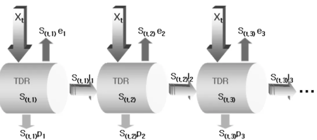
In a dense scenario, the number of events may be huge, so the time points when events happen may be extremely close to one another (i.e., quite successive on the time