Fog Rendering Using Distance-Altitude Scattering Model on 2D Images

(1)

Fog Rendering Using Distance-Altitude Scattering Model on 2D Images

Hochang Lee^†, JaeNi Jang^††, KyungHyun Yoon^†††

ABSTRACT

We present a fog generation algorithm in 2D images. The proposed algorithm provides a scattering model for the approximated calculation of fog density. The scattering model needs parameters of distance and altitude information. However, 2D images do not include that information, so that we calculate them from the depth information generated in an interactive manner, and estimate the scattering factor by using the scattering model. Then we generate fog effect on an input image using the scattering factor by distance-oriented selection blur and color blending. With the algorithm, we can easily create the fog-effected images and fog generated animation from 2D images.

Key words: Picture/Image Generation; Rendering; Fog Effect.

※ Corresponding Author : Kyunghyun Yoon, Address : (156-756) Computer Graphics Lab. Dept. of CS&E, Chung-Ang Univ. 221, Hukseok-Dong, Dongjak-Gu, Seoul, Korea, TEL : +82-2-820-5308, FAX : +82-2-824- 3018, E-mail : [email protected]

Receipt date : Oct. 31, 2011, Revision date : Dec. 21, 2011 Approval date : Dec. 21, 2011

†††School of Computer Science & Engineering, ChungAng University, Korea

(E-mail: [email protected])

†††Convergence R&D Lab. LG electronics Inc.

(E-mail: [email protected])

†††School of Computer Science & Engineering, ChungAng

University, Korea(E-mail: [email protected]) Fig. 1. Fog effect in industry. (left) Game, (right) music video.

1. INTRODUCTION

The simulation of natural phenomena is one of the important research fields in computer graphics.

In particular, aspects such as sky, clouds, water, fire, trees, smoke, terrains, desert scenes, snow and fog are indispensable for creating realistic images.

In this Paper, we focus on the fog effect. Fog is a natural phenomenon that light is scattered by at- mospheric aerosol. However, fog is also made arti- ficially for some purposes. Especially in visual industry, fog effects are used to create a specific sense of mood or atmosphere not only by making artificial fog actually in the scene but also by pro- ducing fog effects on pictures [1-2] (Fig. 1).

Notable examples of the fog effect are a fog ma- chine and a camera with a fog or a diffusion filter.

Both methods enable low-cost shooting. However, they have limitations that the features of fog effect such as form, volume, and density are fixed at the same time of the shooting and can never changed.

Furthermore, the former is not applicable to every scene, and the latter is only for haze level effect.

To overcome such restriction, CGI (Computer Generated Imagery) is used which has the secon- dary effect on images. There are largely two methods of creating fog with CGI. One is to use image processing tools on 2D images, and the other is to simulate fog using 3D models. In 2D methods, all the features of the effects are determined by the user so that the user’s skill is very important. On the other hand, they are controlled by geometric information and some parameters in 3D methods.

(2)

Accordingly, the automatic simulation is possible by just deciding some parameters with 3D methods.

A 2D image has no geometric information as a 3D model does. The information is essential to simulate the fog. Even though the method of automatic fog rendering provides reliable results and needs shorter work time, it is useless in 2D images.

To address this problem, we suggest a new ap- proach for automatic fog rendering that can be applicable to 2D images. First, we segment an input image using interactive graph-cut algorithm, and make a depth map. Then we calculate the distance-altitude information through the depth map, and user-defined parameters. After the creation of geometric information 2D lacks, the information estimates the scattering factor using the proposed scattering model. Lastly, we generate the fog rendering result using distance-oriented selection blur and color blending.

The main contributions of this article are twofold. First, we introduce a method which enables the fog rendering on 2D images by format- ting the geometric information with simple UI.

Second, we define a distance-altitude scattering model, which is simple but generates acceptable results.

2. RELATED WORK

Fog rendering is a very classical topic in computer graphics. It has been used almost essentially to increase the reality, and it offers depth culling to the scene created by computer graphics technology.

Reeves [3] proposed the particle system to ren- der fuzzy objects, and Kajiya et al. [4] applied it to ray tracing using the light scattering equation.

Particle-used rendering enables the acquisition of realistic results. However, very high cost is needed, and many researches to improve processing speed have been progressed [5-8].

In this paper, we calculate the scattering factor

and use image processing method through the proposed distance-altitude scattering model to ex- press fog effect in a 2D image instead of simulating by particle system.

3. FOG GENERATION ALGORITHM

3.1 Distance-altitude information

Fog appearance is dependent on the distance from a camera to the terrain, the condition and density of atmosphere. As the distance gets fur- ther, we get more scattering. Also, as a worse condition if there are more particles of moisture or dust in the air, it results more scattering. Besides, the degree of scattering is directly proportional to the degree of density. Accordingly, scattering happens less in high altitude area due to lower air density compared to near ground [1].

For automatic fog rendering, above features are necessary. However, the features are unobtainable in 2D images. Thus, we create the approximated distance-altitude information through the follow- ing process.

1. Segment an input image into several areas by using interactive graph-cut algorithm [9].

2. Allocate depth values to each area relatively.

3. Calculate each pixel’s distance and altitude information by using the created depth map and user-defined parameters.

At first, we use the graph-cut algorithm for efficient segmentation. This algorithm is a technique for general purpose interactive segmentation of N-dimensional images. The user marks certain pixels as an “object” or a “background” to provide hard constraints for segmentation. Additional soft constraints incorporate both boundary and region information. The Graph cuts are used to find the globally optimal segmentation of the N-dimensional image.

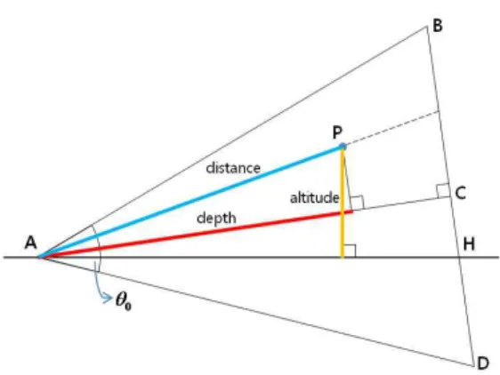
In third process of above, the shooting is sup- posed to be done in the condition of altitude and lateral horizontal state in the input image. The pa-

(3)

rameters are as listed.

y0 : y coordinate of the horizontal line in the image

q

0: the vertical angle of view of camera We can reconstruct the view-frustum of shooting with two parameters as Fig. 2. On the supposi- tion that A is homologous with the site for shooting, ^AC with shooting direction, ^AC with the maximum value of developed depth map, the hori- zon H can be estimated by y⁰ and

q

0. And then,

∆ABD could be considered as the view-frustum of camera. Accordingly, each pixel’s distance and altitude information can be figured out by using the given depth map, y⁰, and

q

0_.

Fig. 2. The reconstruction of view-frustum.

3.2 Estimation of the scattering factor

Beer-Lambert law Eq. (1) [10,11] represents the scattering of light in the air, and frequently used in the computer graphics for the rendering of scattering effect.

scl

e I I

T = /

₀

=

^-^s (1)

This law defines the transmission rate as the ratio of the transmitted intensity to the intensity of incident light, which is expressed as exponential function through scattering coefficient of medium and the thickness of mediuml . And the increase of

s

^sc _and l brings the decrease of T.

In the landscape scene, the scattering coefficient

for each pixel is changed due to the altitude. For this, Equation 2 defines a new scattering model dependent on distance-altitude and controllable with few parameters.

) ( ) ( ) 1

( e ^sc^R^k e ^h^H^k

f = - ^-^b ^b (2)

Equation 2 determines the scattering factor f considering distance and altitude. The range of f is ⁰^{£ f} ^£¹. When the f value is higher, the scattering degree is strengthened. ^s^sc and l in equation 1 are homologous with b^sc andR(k) in Eq. (2). The distance coefficient bsc and the distance of each pixelR(k) determine scattering degree due to the distance. In addition, the altitude coefficient bh and the pixel’s altitude H(k) influences on scattering degree to the altitude. b^sc and bh are real number bigger than 0. When b^sc becomes greater, the scattering factor becomes smaller. When bh becomes greater, the scattering difference by altitude becomes greater. Fig. 3(b) is the visualized image of f calculated from the input image and the corresponding depth map (Fig. 3(a)).

bsc in equation 2 has a constant value. However, the air distribution is not consistent in real world, so fog develops as inhomogeneous aspect. Particle simulation is required for reflecting such charac- teristics, but it demands high calculation cost.

We multiply Perlin Noise N(k) _by bsc to get similar effect with less expense as Eq. (3) [12-13].

) ( ) ( )

(

)

1 ( e

^sc^N ^k^R ^k

e

^h^H ^k

f = -

^-^b ^b ⁽³⁾

Fig, 3(c) is the visualized image of Perlin Noise, and Fig. 2d is visualized image off calculated by Eq. (3).

3.3 Application of fog effect

The scattering of light makes the edges of distant objects blurred and the chrome of them reduced. We get the former effect by using distance-oriented selection blur and the latter effect by using color blending that uses f.

(4)

(a) The input and depth (b) Map by equation 2 map

(c) The Perlin noise (d) Map by equation 3 image

Fig. 3. The estimation of the scattering factor with/

without Perlin noise, (a) The Input image, (b) Map by Eq. (2), (c) The perlin noise image, (d)Map by Eq. (3)

(a) The result of distance-oriented Gaussian blur

(b) the result of distance-oriented selection blur Fig. 4. Modified blur kernel, (a) The result of dis-

tance-oriented Gaussian blur, (b) the result of distance-oriented selection blur

For the effect of edge blurring, we use Gaussian blur on the input image. We set the size of Gaussian kernel firstly by the size of the input image. Then we control the size of the kernel proportional to f because the light is more scattered, and the edges are more blurred. As we multiply kernel size andf, we generate the weaker blurring effect in the spot where scattering is smaller and the stronger effect in the spot where scattering is greater. However, it’s not enough to adjust the size of the kernel. When the distant and close objects in the input image are blurred together, the pixels are influenced by the color of the close objects due to its large sized kernel.

As the result, the color of the close objects is speeded across own edges (Fig. 4(a)). Accordingly, we use distance-oriented selection blur to get rid of such phenomenon and to blur only the edge of distant view. In case of blur kernel lying from distant objects to close objects seen in Figure 3, we set the given weight to pixels of close objects rath- er than in the center as 0 for the results of blur should not to be affected (Fig. 4(b)).

This method is helpful for the prevention of the color of close objects from spreading to distant objects, and for selective application of blur to distant objects.(This method is helpful to prevent the spread of color from close objects to distant objects. It is also helpful for selective application of blur to distant object) Color blending of each pixel by Eq. (4) is done for the application of

(5)

(a) The rendering result by equation 2 (b) The rendering result by equation 3

Fig. 5. Rendering Results according to Perlin Noise (parameters: (a) b_sc=3.3,b_h=0.6,C_f =RGB(255,255,255) _(b) )

255 , 255 , 255 ( ,

6 . 0 ,

10 _h C_f RGB

sc = b = =

b _).

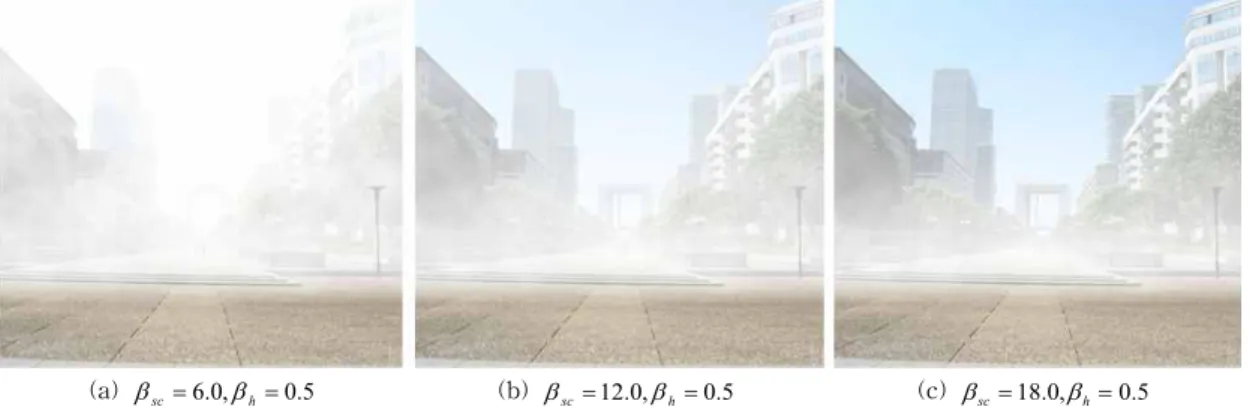
(a) bsc=6.0,bh=0.5 (b) bsc=12.0,bh=0.5 (c) bsc=18.0,bh=0.5 Fig. 6. The results using various distance coefficients with C_f =RGB(255,255,255)

chrome lowering after the distant view being blurred by distance-oriented selection blur.

) 0 1

( f C

C f

C_s= × _f+ - × (4)

C0is the image color of which selection blur being applied,Cfis blending color andCsis the color obtained from scattering effect.

4. EXPERIMENTAL RESULTS

We experimented with different parameter values and target images & video. Including pre-processing time, it takes about 4s for a VGA image size. We used a Pentium 2.8 GHz quad-core PC with 4 GB of memory to produce the results shown in this paper.

Fig. 5-(a) is the result without Perlin Noise, and Fig. 5-(b) is the result with Perlin Noise. Figure 5-(a) is the identical results of the scattering factor of the things at the same distance-altitude due to the application of identical scattering coefficient to identical distances; On the other hand, Figure 5-(b) shows more natural result through the application of Perlin noise.

Fig. 6 is the results of various scattering coefficient. As b^sc get bigger, the fog gets thicker.

In addition, Fig. 7 shows that as

b

^h gets bigger, the change in effect to the altitude gets greater.

Fig. 8 shows the result with various fog colors using equation 4. With the control of the fog color, we can generate lots of results with intended mood.

(6)

(a) b_sc=15.0,b_h=0.0 (b) bsc=15.0,bh=0.5 (c) b_sc=15.0,b_h=1.0 Fig. 7. The results using various altitude coefficients with C_f =RGB(255,255,255)

(a) ^fc=^RGB⁽¹²⁰^,¹⁰⁰^,⁸⁰⁾ (b) ^fc=^RGB⁽²⁰⁰^,¹⁶⁰^,¹²⁰⁾ (c) ^fc=^RGB⁽²⁰⁰^,²⁰⁰^,²⁰⁰⁾ Fig. 8. The results by various fog color with b_sc=10.0,b_h=0.6

Animation can also be created by using 3D Perlin noise. The fog can be blown by wind when the user moves the noise the result fog can be cleared out through the adjustment of the scattering coefficient. The images in Fig. 9 are frames ordered by time in a fog animation generated by the decrement of the distance scattering coefficient.

It shows the scene which fog is cleared out.

4.1 Conclusion and Future work

We present a fog rendering method for 2D images. It is the creation of geometric information 2D lacks through UI. Then we use the information

to the defined distance-altitude scattering model for fog creation. We create fog-effected images using suggested method. Besides, fog animation is made through a slight parameter adjustment and 3D noise application.

The major contribution of this paper lies in easy application of fog effect to images. Our algorithm enables fog creation just through intuitive and simple operation.

Fog animation for motion picture is frequently used in the visual industry. However, the presented method is hard to apply on video, for it requires a great deal of user interaction in creating depth.

(7)

Fig. 8. The frames of fog animation generated by adjustment of bsc with 3D Perlin noise.

Thus, the consideration of video depth creation method is necessary. Finally, we will apply various NPR effect such as [13] based on our algorithm.

ACKNOWLEDGEMENT

This work was supported by a Korean Science and Engineering Foundation (KOSEF) grant fund- ed by the Korean government (MEST)(No.

20110018616).

REFERENCES

[ 1 ] M. Kemp, The Science of Art (NH: Yale University Press, 1990).

[ 2 ] M. Sturken and L. Cartwright, Practices of Looking : an Introduction to Visual Culture (NY : Oxford University Press, 2009).

[ 3 ] W.T. Reeves, “Particle Systems - a Technique for Modeling a Class of Fuzzy Objects,”ACM Transactions on Graphics (TOG), Vol.2, No.

2, pp. 91-108, 1983.

[ 4 ] J.T. Kajiya and B.P.V. Herzen, “Ray Tracing Volume Densities,”ACM SIGGRAPH Com- puter Graphics archive, Vol.18, No.3, pp. 165- 174, 1984.

[ 5 ] D.S. Ebert and R.E. Parent, “Rendering and Animation of Gaseous Phenomena by Com- bining Fast Volume and Scanline A-Buffer Techniques,”The 17th annual Conference on Computer Graphics and Interactive Techni- ques, pp. 357-366, 1990.

[ 6 ] T. Nishita and Y. Dobashi, “Modeling and Rendering of Various Natural Phenomena Consisting of Particles,” P roc. of Computer Graphics International 2001, pp. 149-156, 2001.

[ 7 ] M.J. Harris and A. Lastra, “Real-Time Cloud Rendering,”Computer Graphics Forum, Vol.

20, No.3, pp. 76-85, 2001.

[ 8 ] V. Biri, S. Michelin, and D. Arquès, “Real- Time Animation of Realistic Fog,”Thirteenth Eurographics Workshop on Rendering, pp. 9- 16, 2002.

[ 9 ] Y.Y. Boykov and M.P. Jolly, “Interactive

(8)

Graph Cuts for Optimal Boundary & Region Segmentation of Objects in N-D Images,”In P roceedings of the 8th IEEE International Conference on Computer Vision(ICCV’01), pp.105-112, 2001.

[10] J. T. Houghton, The Physics of Atmospheres 3rd Edition (NY: Cambridge University Press, 2002).

[11] J. D. J. Ingle and S. R. Crouch, Spectrochem- ical Analysis (NJ: Prentice Hall, 1988).

[12] K. Perlin, “Improving Noise,”ACM Transac- tions on Graphics (Proceedings of SIGG- RAPH 2002), Vol.21, No.3, pp. 681-682, 2002.

[13] J. Jang, S. Ryoo, S. Seo, H. Lee, and K. Yoon,

“A Study on Aerial Perspective on Painterly Rendering,” J ournal of Korea Multimedia Society, Vol.13, No.10, pp. 1474-1486, 2010.

Hochang Lee

2006 Received B.Ss degrees in the Department of CS &E from ChungAng Univ.

2008 Received M.Ss degrees in the School of CS&E from ChungAng Univ.

2008～Current Candidate Ph.D student in ChungAng Univ.

Research interest : Computer Graphics, NPR, Image stylization, GPGPU

JaeNi Jang

2009 Received B.Ss degrees in the Department of CS&E from ChungAng Univ.

2011 Received M.Ss degrees in the School of CS&E from ChungAng Univ.

2011∼Current Researcher inConvergence R&D Lab.

LG electronics Inc.

Research interest : Image based rendering, NPR

KyungHyun Yoon

1980 Received B.Ss degrees in the Department of CS from ChungAng Univ.

1983 Received M.Ss degrees in the Department of CS from ChungAng Univ.

1983～1985 Researcher in Korea Electrotechnology Research Institute

1988 Received M.Ss in the Department of CS from University of Connecticut

1991 Received Ph.Ds in the Department of CS from University of Connecticut

1991～Current Professor in the School of CS&E, ChungAng Univ.

Research interest：Computer Graphics, GIS, Image- Based Rendering, NPR