Direct Controller for Nonlinear System Using a Neural Network
Cheol-Soo Bae
*· Young-Cheol Park
**· Kee-Hwan Nam
***· Yong-Seok Kang
****Tae-Woo Kim
****· Suen-Ki Hwang
*****· Hyon-Yul Kim
**· Moon-Hwan Kim
******Abstract
In this paper, a direct controller for nonlinear plants using a neural network is presented. The controller is composed of an approximate controller and a neural network auxiliary controller.
The approximate controller gives the rough control and the neural network controller gives the complementary signal to further reduce the output tracking error. This method does not put too much restriction on the type of nonlinear plant to be controlled. In this method, a RBF neural network is trained and the system has a stable performance for the inputs it has been trained for. Simulation results show that it is very effective and can realize a satisfactory control of the nonlinear system.
Keywords : RBF, neural network, nonlinear system, direct controller, complementary signal
* 교신저자 관동대학교 의료공학과 교수 ([email protected])
** 관동대학교 정보통신공학과 박사과정
*** (주)삼형전자 선임연구원
**** 한국폴리텍Ⅲ대학 교수
***** 한국폴리텍Ⅳ대학 교수
****** 한국전파기지국(주) 기술연구소장
접수일자:2011년 12월 20일, 수정일자 : 2012년 1월 12일, 심사완료일자:2012년 1월 20일
1. Introduction
The conventional design methods of a control system often require the construction of a math- ematical model describing the dynamic behavior of the plant to be controlled. When such a mathematical model is difficult to obtain due to uncertainty or complexity of systems, these con- ventional techniques based on a mathematical model are not well suited for dealing with.
Artificial neural network techniques have been suggested for identification and control of non- linear plants for which conventional techniques
of control do not give satisfactory performance, such as the accuracy in matching the behavior of the physical system.
A good method of applying neural networks for control must have the following properties:
1. It must be applicable to nonlinear plants, since there are already good methods of control for linear plants.
2. It should not put too much restriction on the type of nonlinearity that it can handle.
3. It is preferable to have an Unsupervised
Learning method for the neural network because
the desired output form of a system for a given
input may be known, but the input form of a plant that produces that desired output is not generally known. Unsupervised Training can avoid identification of the plant or its inverse model, which is generally not easy to obtain.
4. The system should be stable at least for the class of inputs it has been trained for.
5. In most cases open loop performance of a plant can be observed and a approximate con- troller can be devised for that. It would be de- sirable if we could put as much knowledge as possible in the design of this controller and only leave the extra fine tuning to the neural net- work controller.
According to the above requirements, a direct auxiliary controller for nonlinear plants using neural network is presented.
2. Controller Design
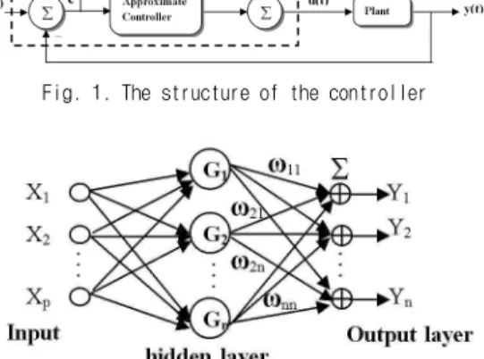
The controller presented here is composed of an approximate controller and a neural network auxiliary controller. The structure of controller is shown in figure 1. The approximate controller gives the approximate performance and the neu- ral network auxiliary controller is used for the purpose of further fine tuning.
The approximate controller can be a PID or any other conventional controller. It can be de- signed by using the known dynamics of non- linear plant. The neural network employed in this scheme is an Radial Basis Function Network (RBFN). It produces the complementary signal to further reduce the error e between output y and the reference input r. The struc- ture of RBFN is showed in Figure 2. It is a network with two layers, a hidden layer of radi- al basis neurons and an output layer of linear neurons. A common choice for the basis function is a Gaussian given by the (1).
Where Ci represents the center of the basis
function and σ denotes its width. The norm ||•
|| in equation can be expressed by Euclidean distance. The weights and biases of each neuron in the hidden layer define the position and width of a radial basis function. Each linear output neuron forms a weighted sum of these radial basis functions. With the correct weight and bias values for each layer, and enough hidden neurons, a RBFN can fit any function with any desired accuracy. The advantage of the RBFN is its rapid learning, generality and simplicity.
RBFN finds the input to output map using local approximations. It can be trained faster than BP and have none of BP’s training problems such as saturation and local minima.
Fig. 1. The structure of the controller
Fig. 2. Radial Basis Function Network
In the RBFN training stage we first observe
the performance of the system with the approx-
imate controller for a certain period of time and
measure the range of error between the output
of the plant and desired output. Then we divide
this error span into certain sections and for each
section we perform a perturbation test: We in-
creased the input to the plant by δe whenever
total square error between the output of the
plant and desired output falls within a specified
region. If this change of the input results in a lower value of the total square error, we modify the output weight of the neural network con- troller to work accordingly. This action is con- tinued for all sections and the whole process is repeated until no modification can reduce the error.
Taking an overlapping Gaussian activation function for kernel units supposedly provides a smoother response and better generalization. But in our case the amount of interference was so high and we obtained a better performance with non-overlapping regions. Nevertheless, smooth- ness of the output can be enhanced by dividing the correction for each section by modifying the cost function used for training from J=∑e2 to J=∑(enew2+k(enew -eold)2) for k<1.
During the training stage, each time only one kernel unit responds and one weight is adjusted, This results in a shorter training time compared with Multi-layer Perception (MLP) type networks. Since weights are adjusted by a small value δ each time, the number of necessary iterations depends on the size of error or the accuracy of the approximate controller.
The point that makes this method different is the way in obtaining the necessary corrections, which is based on the effect of weight perturba- tion on the total square error for a certain peri- od of time. Perturbing the weights of a network is used in Madaline Rule III (MR III) training for analog implementation of neural networks.
Because this method does not need prior knowl- edge about the transfer characteristics of the computing devices, it is not affected by the ef- fects of neuron to neuron variations. Training the network based on its instantaneous result of the error will cause instability when used in a feedback loop. The performance of the system here is observed for a certain period of time and if any adjustment for any given amount of error increases the total square error, it would not be
accepted. This proves the stability of the system for the class of inputs it has been trained for.
Generally optimization methods based on pa- rameter perturbation are bound to failure when many parameters are involved in perturbation and that is because of the moving target effect of the other parameters. It is not the case in the proposed system for which only one or few re- lated parameters are active at each time. At present, methods for directly adjusting the con- trol parameters based on the output error are not available. The work presented in this paper is a step toward direct adaptive control.
3. Simulation Study
Different nonlinear systems were considered to evaluate the effect of the proposed method.
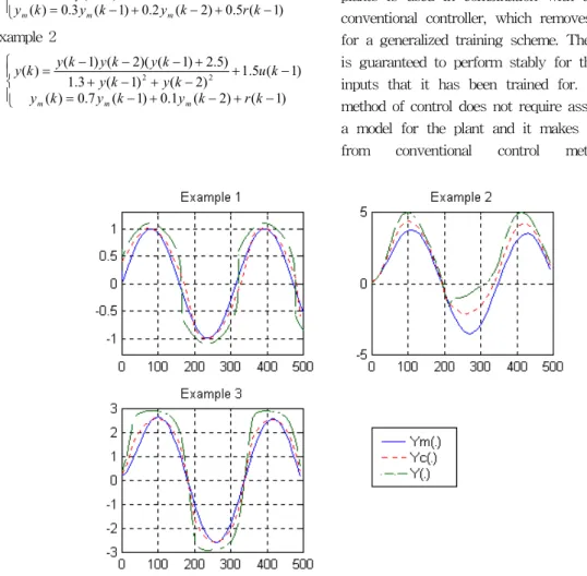
Figure 3 gives the effect of controller when it is used for three different nonlinear plants. In this figure , y(.) denotes the plant output without controller, ym(.) denotes the desired output , r(.) denotes the reference input and yc(.) denotes the output of the plant with controller. An RBF type network with 30 kernel units each sensitive to different ranges of error were used. Input weights and activation function of the units were fixed. Output weights were perturbed and adjusted according to the effect of perturbation on the total square error for 400 sampling time.
For a sinusoidal input (r(k)=sin(k/50)) and per- turbation amount of δ=0.1, the amount of reduc- tion in aggregated square error for a full cycle of input is example 1:from 3.69 to 1.33, example 2:from 105.84 to 26.44 and example 3:from 32.11 to 4.56. To observe the learning and general- ization capability of the system, the controller was trained on a step response and its perform- ance was observed on the sinusoidal input.
Training the network with different types of in-
put will enhance the generalization capability of
Fig. 3. Ym(.) is the output of the reference model, Y(.) is the output of system without NNC and Yc(.) is the output of system without NNC in the example1,2 and 3.
the system.
Example 1
ï î ï í ì
- + - +
-
=
- - +
+
= -
) 1 ( 5 . 0 ) 2 ( 2 . 0 ) 1 ( 3 . 0 ) (
) 1 ( 5 . ) 0 1 ( 1
) 1 ( 2 . ) 1
(
2k r k
y k
y k y
k k u
y k k y
y
m m
m
Example 2
ï î ï í ì
- + - +
-
=
- - +
+ - +
+ - -
= -
) 1 ( ) 2 ( 1 . 0 ) 1 ( 7 . 0 ) (
) 1 ( 5 . ) 1 2 ( ) 1 ( 3 . 1
) 5 . 2 ) 1 ( )(
2 ( ) 1 ) (
(
2 2k r k y k
y k y
k k u
y k y
k y k y k k y y
m m
m
Example 3
) ) exp(
1 3 6 ) ( (
) 1 ( ) 2 ( 2 . 0 ) 1 ( 48 . 0 ) (
)) 1 ( 1 . 2 ) 2 ( 2 . 0 ) 1 ( 5 . 0 ( ) (
x x sat
k r k y k
y k y
k u k
y k
y sat k y
m m
m
- + + - º î í
ì
- + - +
-
=
- + - + -
=
4. Conclusions
A neural network controller for nonlinear plants is used in combination with an existing conventional controller, which removes the need for a generalized training scheme. The controller is guaranteed to perform stably for the class of inputs that it has been trained for. Using this method of control does not require assumption of a model for the plant and it makes it different from conventional control methodologies.
Furthermore, since training of this network does
not require backpropagation of error, it makes
direct adaptive control possible, a structure be-
yond the capabilities of backpropagation based
on neural networks. The structure used here can
be view as a fuzzy controller implementation for
which the control actions or rules which depend
on the error between the plant output and the desired output are deduced in training time. It can also be viewed as a gain scheduling adap- tive controller which can work for any unknown plant with no attempt to linearize the system at each region.
References
[1] J. Moody and C. J. Darken, “Fast learning in Networks of Locally-Tuned Processing Units,” Neural Computation, Vol. 1, pp.
281-194, 1999
[2] D. Andes, B. Widrow, M. Lehr and E. Wan,
“MR III:A Robust Algorithm for Training Analog Neural Networks” International Joint Conference on Neural Networks,1999 [3] K. S. Narendra and K. Parthasarathy,
“Identification and Control of Dynamical Systems Using Neural Networks” IEEE Trans on Neural Network Vol.1 No.1, pp.4-27, 2003
[4] M. M. Gupta and D. H. Rao, “Dynamic Neural Units in the Control of Linear and Nonlinear Systems,” In Proceedings of the International Joint Conf. On Neural Networks, June 2004, pp.100-105
[5] G. A. Montague, M. J. Willis and A. J.
Morris, “Artificial Neural Network Model Based Control,” Automatic Control Conference, 2005
[6] Howard Demuth, Mark Beale, “Neural Network ToolBox for Use with MATLAB,”
The MathWorks Inc., 2006
[7] Chen S, Billing S A, “Grant P M. Recursive Hybrid Algorithm for Nonlinear System Identification using Radial Function Network,” Int. J Control,2007,55(5):1051-1070 [8] 박호식, 남기환, 정하영, 배한별, 배철수, “신경 망을 이용한 물체의 방향검출,” 한국정보전자통
신기술학회 추계학술대회발표집, pp. 256-259, Vol 4, No2, 2011
저자약력