Development of Gas Turbine Simulation Program Based on CFD

Development of Gas Turbine Simulation Program Based on CFD

Sangwook Jin^*, Jaemin Kim^**, Kuisoon Kim^**, Jeong-Yeol Choi^**, Iee Ki Ahn^*** and Soo Seok Yang^***

*Research Institute of Mechanical Technology

**Department of Aerospace Engineering, Pusan National University

***Aeronautics Program Office, Korea Aerospace Research Institute

Pusan National University, 30 Jangjeon-dong, Geumjeong-gu, Busan, 609-735, Korea [email protected]

Keywords: Engine simulation, Propulsion system, Gas Turbine engine, Computational Fluid Dynamics Abstract

A program based on a 2-D CFD code has been developed to simulate a gas turbine engine. 2-D Navier-Stokes implicit code with k-ω turbulent model is used in compressor and turbine. Lumped method chemical equilibrium code with 10 species of molecular is applied to combustor with assuming perfect mixture and 100% combustion efficiency at constant pressure state. Fluid properties are shared on interfaces between engine components. Compressor supplies outlet temperature and pressure to combustor.

At the same time, combustor also carries temperature and pressure to turbine. The back pressure of compressor outlet is transferred by inlet pressure of turbine. Unsteady phenomena in rotor-stator are covered by mixing-plane method. The running condition of engine can be determined only by given the inlet condition of compressor, the outlet condition of turbine, equivalence ratio and rotating speed.

Introduction

The basic theory of contemporary gas turbine engine was suggested by English man, John Barber in 1791. But after becoming 1937, the engine generating useful power was made by Frank Whittle in England^1-

2). There were also continuous efforts to design and develop a new gas turbine engine only depending on simple “cycle analysis.” This cycle analysis needs performance maps of engine components; compressor, combustor and turbine, which can be attained by numerous tests in various conditions. After all components go through the complex steps of design, hand-made and test, the final version of engine could be accomplished. By the way, during design engine, there’s no performance map so the engineers use another one in similar condition and it requires several times of revision due to the use of incorrect data.

In early time, it was “streamline curvature method”

for the major analysis way to estimate the performance of engine by using computer. Streamline curvature method assumes some facts and contains errors. Owing to a computer’s improvement in its calculation speed and memory, 3-D CFD method is utilized in multistage compressors and turbines that it can be used to optimize the design of blades. But the separated design of engine components might be easy to omit the interactions between them. It causes the

performance estimation. To overcome this problem, developers are trying to use a full engine simulation.

The activities to develop a full engine simulation system are implemented by large two groups; North America and Europe. In USA, a NPSS (Numerical Propulsion System Simulation) project was started from 1987. In 1999, it released the result of the whole simulation of the GE90 turbo fan engine only taking 15 hours which meant its goal to make the possible of

“over-night” calculation and practical use^3-6). The PROOSIS(Propulsion Object Oriented Simulation Software) in Europe is actually based on cycle analysis program. Almost all the countries in Europe have their own developed cycle analysis programs. As standardizing and unifying them with advanced functions; CFD and multidisciplinary analysis, they try to reduce the effort to make a gas turbine engine from 20057-8).

Even through these kinds of research has been continued for long time since it started, to get the specific information of them is very hard for a late developer because its related technology is regarded as confidential one. This research is implemented by focusing on getting the basic technology about a full engine simulation system and shows the analysis of separated and combined components of engine.

Methodology

Performance data of compressor and turbine come from the result of CFD code consisted of 2-D Navier- Stokes equation. The temperature of combustor outlet is generated by chemically equivalent reaction of methane gas as regarding it 0-D point. This program can be completed as based on interaction process between components.

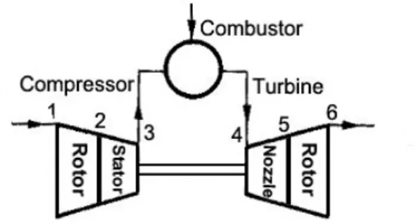
Figure 1 Engine Structure

Algorithm of Program

The computer program of engine consists of module components as exchanging the boundary condition between them. The nomenclature of engine parts is suggested in figure 1. The air goes through the compressor, the entrance 1 to exit 3 with pressurization then burns through 3 to 4 with mixture of fuel. Burned gas speeds up at the entrance 4 of turbine and expands at the outlet of turbine 6.

Above procedures are translated to a computer program flowchart in figure 2. The main code manages and calls the subroutine modules from compressor to turbine as checking their convergence.

After converged, post process converts all data to be ready to use it.

Figure 2 Program Flowchart

The boundary conditions between engine components are divided into two forms; specified and extrapolated ones. In 2-D case, the total condition of entrance and exit is 4. In subsonic case at entrance, three of them are specified and the rest is extrapolated by internal properties. And three extrapolated and one specified conditions are given to the boundary condition at exit. If we limit the running condition as subsonic case, the 3-specified condition at compressor inlet can be density and velocity with angle which make it up the mass flow rate, then 1-specified condition at turbine outlet; back pressure is the exit condition of engine. On the interfaces of engine components, the vectors of velocity for x, y-directions and the density are the exit condition, and the pressure is the outlet condition. The assumption regarding combustor as 0-D only occurs temperature increase depending on the equivalence ratio of air-fuel at constant pressure after leaving compressor. Because of that process, if we use ideal gas equation with the exit pressure and temperature, it can be attained the inlet density. The velocity of turbine inlet can be derived by the area of turbine with density according as the mass flow is constant. If we summarize above all procedure, we could know the fact that the inlet condition of compressor and outlet condition of turbine with equivalence ratio consist of all condition of engine.

The calculation method of compressor and turbine

Governing equation and turbulent model

To analyze the viscous flow in compressor and turbine, 2-D Navier-Stokes equation is introduced⁹⁾. To solve these equations, Roe’s upwind scheme for space and LU-SGS(Lower Upper-Symmetric Gauss Seidel) in time step are used with k-ω SST turbulent model which is combination of k-ω model that gives good agreement without using complex wall function and k-ε model which is not effected by inlet ambient flow.

Verification of code

The four European wind tunnel experiments for VKI (von Karmann Institute) turbine cascade conducted by Kiock et al are prevalent as a validation case in 2-D computational fluid dynamics¹⁰⁾. To verify this code, we used their experimental data at the case of inlet velocity M 0.282 and outlet velocity M 0.78 as well as M 0.96. The 141x51 H-type grid was made to calculate it at the same condition and it shows good agreement in subsonic and transonic cases as following results on the figure 3 and 4.

Figure 3 Isentropic Mach No. Distribution on Blade Surface, M_ex =0.78(left) M_ex =0.96(right)

Figure 4 Mach No. Contour And Schlieren Picture at M_ex =0.96, Re_ex=8.8×10⁵

Rotor-Stator Model

There are three types of unsteady flow mechanism between blade rows by the rotation of rotor blade row.

They are potential flow interaction, wake interaction and shock wave interaction. Each of them is related to inviscid flow, viscous flow and shock system, respectively. The unsteady fully coupled blade row (FCBR) techniques require too much time and enormous computer resources while they are the most accurate solution to predict all the phenomena. To overcome this matter, steady coupled row (SCBR) techniques are implemented through the use of mixed- out steady boundary conditions. SCBR needs relatively small amount of time and resource even though some physical processes such as wake mixing and migration, acoustic interaction and other unsteady effects are ignored. But it is reported for SCBR to provide a reasonable representation of FCBR results^11-

12). There are two representative method of SCBR; the mixing-plane method and frozen rotor method. First one is another name of averaging-plane method which is developed by Dawes et al. This method averages the properties of flow at the exit of rotor for span wise direction then gives these values to the inlet condition of stator. But there is possibility to omit the physical phenomena due to averaged flow. The second one, frozen rotor method is originated from Adamcyzk¹³⁾’s average-passage method. That is actually unsteady solution but it doesn’t consider the rotation of rotor that its result can be meaningless as unsteady one¹⁴⁾. Both of them arrange the reasonable boundary condition on interface and calculate all the cascades at the same time, so the interaction is recognized on it except for important phenomena; the mixing and spread of wake and acoustic interaction¹⁴⁾. In case of the frozen rotor method needs the same geometric boundary between blade rows, and they should have same period. Besides, pitch also must be same at their channel. By the way, the mixing-plane method averages all properties of flow, and it does take into consideration for their geometrical set, pitch and period. Consequently, it is easier than frozen rotor method to apply to a code. So, in this study, the second one is selected to solve the interaction problem between rotor and stator.

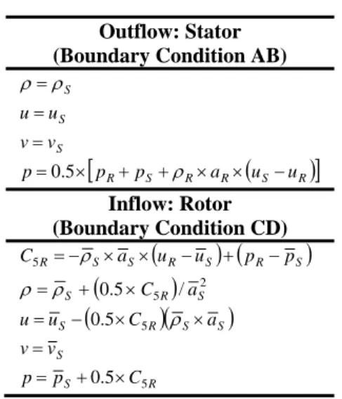
Figure 5 Stator Rotor Block Diagram

Table 1 Characteristic Boundary Condition Outflow: Stator

(Boundary Condition AB) ρS

ρ= uS

u= vS

v=

( )

[pR pS R aR uS uR ]

p=0.5× + +ρ × × − Inflow: Rotor (Boundary Condition CD)

( R S) ( R S)

S S

R a u u p p

C₅ =−ρ × × − + −

(0.5 5_R)/ _S²

S+ ×C a

=ρ

ρ ( )( )

R S

S

S S R S

C p

p v v

a C

u u

5 5

5 . 0

5 . 0

× +

=

=

×

×

−

= ρ

The characteristic boundary conditions are given as following Figure 5 and table 1^12-13). Subscript S and R mean a stator block and a rotor block. And C_5Ris a characteristic value, ‘-’ means an averaged value. This way of setting boundary preserves the non-uniformity spatial details of the flow without the smearing associated the averaging process and allows the continuity of the flow variables at the rotor-stator interface boundary condition¹³⁾.

The Average of Flow Properties

One of averaging method of flow, mixed-out average method averages all the things of flow that it provides totally developed flow at downstream.

Another one, kinetic energy average method makes flow locally constant state that mass, static enthalpy and velocity square term is conserved and static pressure becomes locally averaged value, then averaged pressure omits mixing loss at downstream¹⁸⁾. In order to reduce the loss of physical phenomena, the second method is embedded in program. More specific explanation is showed in following equations.

Velocity square term, metric relation and contra variant velocity are;

2 2

2 u v

V = +

(

)

J= /1 +

ξ ξ η η

η η ξ ξ

Jx Jy Jx Jy

x y y x

=

−

=

−

=

=

(

)

ξ

ξ u v Juy vx U= _x + _y = −

All flux terms are defined as following equations, and integrated along the inlet boundary.

U V d V J vdA V I

U h d h J dA v h I

U v vUd J dA vv I

U u uUd J dA uv I

U Ud J dA v I

n n n n

2 2

1 2

5

0 0

1 4 0

1 3

1 2

1 1

ρ η ρ ρ

ρ η

ρ η ρ

ρ η ρ

ρ η ρ ρ

∫ =

∫ =

=

∫ =

∫ =

=

∫ =

∫ =

=

∫ =

∫ =

=

∫ =

∫ =

=

−

−

−

−

−

First of all, we attain the inverse value of I₁=ρU then the other values can be derived one after another.

( )

2 2

2

1 2 3 2 2 1

5 1 1

I v u

V I I I I

r I =

= +

= +

U I h

U I

v u U

rI v

rI u

y x

/ /

4 0

1 3 2

=

= +

=

=

=

ρ

ξ ξ

Model compressor

The one stage axial compressor comes from PSRC (Pennsylvania State University Research Compressor) only first stage which consists of

2

31 stage containing inlet guide vane. Its geometric data shows in Table 2.

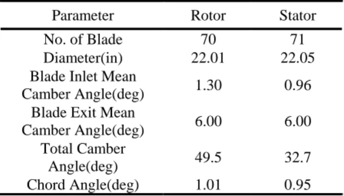
Based on this data, the blade shape is generated as the same way to make airfoil. The pitch between blades set 0.71 for chord length not to calculate from the number of blades and diameter to make it simple computation.

Figure 6 Combination of 141x71 H-Type Gird at Rotor and Stator in Compressor

Figure 6 shows the 141x71 H-type grid of compressor which is combined rotor and stator, respectively. At the middle of one grid row is crossed over to apply mixing plane method.

Table 2 Blade Design Parameter for the PSRC

Parameter Rotor Stator

No. of Blade 70 71

Diameter(in) 22.01 22.05

Blade Inlet Mean

Camber Angle(deg) 1.30 0.96

Blade Exit Mean

Camber Angle(deg) 6.00 6.00

Total Camber

Angle(deg) 49.5 32.7

Chord Angle(deg) 1.01 0.95 Model Turbine

The turbine model comes from LSRR-I (Large Scale Rotating Rig No.1) of UTRC (The United Technologies Research Center). The parametric data of the turbine is listed on table 3. It is the same one which used in the experiment of R. P. Dring et al²⁰⁾. But pitch is changed into 0.71chord length and gab between nozzle and rotor is the same length of chord.

The number of grid is also same with compressor and it is also crossed over at the middle of grid for mixing plane method (figure 7).

Table 3 Airfoil Geometry and Nominal Operating Condition

Parameter Nozzle Rotor

No. of Blade 22 28.

Diameter(ft) 5 5 Stagger Angle(deg) 49.5 32.7

Inflow Angle(deg) 90.0 40.0 Outflow Angle(deg) 22.5 25.5

Figure 7 Combination of 141x71 H-Type Grid at Nozzle and Rotor in Turbine

Combustor

The chemical equilibrium code used in this program does not contain any ejected, mixed and evaporating process. It only calculates the temperature as assuming perfectly mixed and burned gas. This process has benefit to reduce computing time and resources except for non reality. But we can expect the function of a combustor to get the combustor temperature and the increase of mass flow rate with addition of fuel. And it

causes expansion and the increase of axial velocity.

Finally it supplies the energy make a turbine rotate.

Table 4 Comparison of CEA and In-house Code for Mole Fraction of Product According to Temperature and Pressure

CEA In house

code Error Temperature(K) 2318 2318

Pressure(bar) 11 11

Mole Fraction

O

H₂ 0.18577 0.18541 0.19 % CO2 0.08818 0.08761 0.64 % CO 0.00640 0.00693 8.38 % OH 0.00224 0.00195

NO 0.00182 0.00174 4.40 % O2 0.00291 0.00342 17.53 % H2 0.00238 0.00261 9.66 % N2 0.71027 0.7008 0.03 %

O 0.00009 0.00008 11.11 % H 0.00016 0.00016 0.00 % N 0.00000 0.00000 0.00 %

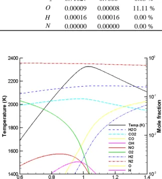
Figure 8 Temperature and Mole Fraction Variation for Equivalence Ratio Change

GaseousCH₄ is the only fuel to be used in this code.

It generates fewer molecules than kerosene series fuels.

It maintains only gas phase. It mean more real than liquid state fuel. Another assumption is that air consists of two molecules; oxygen and nitrogen.

( )

52 . 7 ,

2 ,

1

52 . 7 2 1 76 . 3 2

2 2

2

2 2

2 2

2 4

=

=

=

+ +

→ +

+

N O H

CO N N

N

N O H CO N

O CH

(N_CO N_HO

2

2, and N_N2means the number of mole of subscript molecules)

Theoretical combustion generates only above molecules. But in real case, it produces various gases.

In this case, only 11 species of products

( H₂O,CO₂,CO,OH, NO,O₂,H₂, N₂,O,H,N ) are considered. To verify this combustor, CEA (Chemical Equilibrium and Application) code was utilized. CEA code²¹⁾ has been developed by NASA Glenn Research Center and used to get the chemical components at thermal equilibrium state, the theoretical performance of a rocket, Chapman-Jouguet detonation and the calculation of shock tube problem. Table 1 shows us its reasonable result compared with CEA code.

The temperature and pressure of reaction are 2318K and 11 bar respectively. The major products,

2 2 2O,CO,N

H are almost same mole fractions less than 1 % error between CEA and in-house code. In Fig. 5 show the variation of temperature and mole fraction according to the change of equivalence ratio.

The maximum temperature is observed at the equivalence ration 1.05 and Fig. 5 also present a same tendency.

Model Engine

The specification of engine consisted of 1 stage compressor, 1 stage turbine and 0-D combustor is listed on Table 5. Inflow angle is set due to no inlet guide vane, and mass flow rate is also specified by giving inlet velocity and inlet sectional area. Rotating speed is M 0.3 in compressor and turbine. The equivalence ratio of methane is 0.451.

All the properties are non-dimensionalized by inlet values. The CFL No. of compressor and turbine is set 35 and calculation is done over again until converged as checking inlet total pressure and the difference of density in turbine rotor.

Table 5 Engine Specification

Parameter Compressor Turbine Inlet Angle(deg) 52.97 0.0

Inlet Mach No. 0.282 0.253 Chord Length(m) 0.03 0.03

Blade Height(m) 0.06 0.06 Inner Diameter(m) 0.4 0.4

Rotating Speed(M) 0.3

Equivalence

Ratio(Combustor) 0.451

Result

Following diagram is the convergence of engine during calculation iteration 12,000. It shows us the calculation is almost converged after iteration 9,000 in density case. And inlet total pressure is also converged in near 1.1.

According to the converged data, we checked the state of flow. In compressor made up of rotor and stator in order, air enters into the rotor as inlet angle

° 97 .

52 then flows along the blade. It curves at the middle of blade rows because of adding rotating speed as applying the mixing-plane method. In another words, air flows different coordinate, from relative

one to absolute one as much as the difference of y- direction velocity (figure 10). The distribution of pressure is different from mach No. contour because the averaged inlet pressure of stator applied to outlet pressure condition so it is continuous.

Figure 9 Convergence

Figure 10 Mach No. Contour & Streamline in Compressor

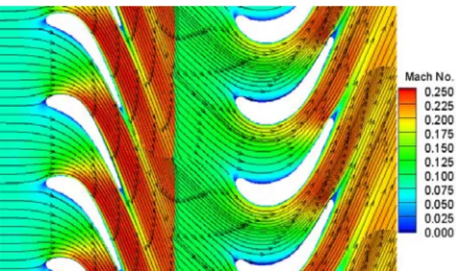
Figure 11 Pressure Contour in Compressor Contrary to compressor, nozzle and rotor consists of turbine in order. Burned gas enters into nozzle with inlet flow angle 0° and is accelerated as losing pressure. Like compressor, there is refraction of streamline at the middle of blade rows due to change

of coordinate (figure 12) and pressure contour is smooth at middle boundary (figure 13).

Figure 12 Mach No. Contour & Streamline in Turbine

Figure 13 Pressure Contour in Turbine

Figure 14 Property Variation Along Rotating Axis

It is showed that the variation of pressure, Mach No.

and temperature along the axis in figure 14. The dash- dot-dot line shows pressure change, it increases in compressor and decreases in turbine opposite trend with Mach No. variation. Finally it leaves engine with atmosphere pressure as 1. While the inlet pressure of compressor and outlet that of turbine must be atmosphere one in real case, 1 stage compressor can not generate sufficient pressure in computational case.

Because of this reason, the entrance pressure of compressor points 1.04 on diagram. The Mach No. is

also changed dramatically in turbine compared with compressor. There is difference of temperature in compressor and turbine but it is not recognized because the amount of temperature variation in combustor is much bigger than the others. The real value of temperature after combustion rises until 1400K.

Conclusion

While the research for the main 3 elements of engine is compressor, combustor and turbine is implemented so many times in industrial field and research groups, it is not so many case in combined cases with considering the interaction of components.

In this point of view, this study is valuable enough and shows us possibility that the combination of solvers can be engine simulator after appropriate interface process to consist of it. In this step, this engine program is imperfect because its module program is not sufficient, only containing 2-D compressor and turbine, 0-D combustor. It means that more study is needed and if this program covers the all weakness of this state, it would be very useful software in industrial field.

Acknowledgement

This study has been supported by the KARI under KHP Dual-Use Component Development Program funded by the MOCIE.

References

1) Kong, C. D., Goo, J. Y., Kim, K. S. and Jeong, H. C., Aircraft Gas Turbine Engine, Dongmyungsa, Seoul, 1999.

2) Hunecke, K., Jet Engine: Fundamentals of Theory, Design and Operation, Zenith Press, 1997

3) Claus, R. W., Evans, A. L., Lylte, J. K., and Nichols, L. D., "Numerical Propulsion System Simulation," Computing Systems in Engineering, Vol. 2, No. 4, 1991, pp.357-364

4) Evans, A. L., Follen, G., Naiman, C., Lopez, I.,

"Numerical Propulsion System Simulation's National Cycle Program," AIAA 98-3113, 1998 5) Lytle, J. K., Follen, G., Naiman, C., Evans, A. L.,

"Numerical Propulsion System Simulation (NPSS) 1999 Industry Review," NASA TM- 209795, August 2000

6) Naiman, C. G., "Numerical Propulsion System Simulation Architecture," AIAA/

ASME/SAE/ASEE 40th Joint Propulsion Conference and Exhibit, June 2004

7) Momsi, P., "VIVACE: Overview", VIVACE Forum 1, September 2005

8) VIVACE Project, http://www.vivacepro ject.com/

9) Choi, J. Y., Superdetonative Mode Starting Process of Supersonic Combustion Ram Accelerator, Ph. D. Dissertation, Seoul National University, 1997

10) Kiock, R., Lehthaus, F., Baines, N. C., Sieverding, C. H. "The Transonic flow Through a Plane Turbine Cascade as Measured in Four European Wind Tunnels," Journal of Engineering for Gas Turbines and Power, Vol. 108, April 1986

11) Dorney, D. J., Sharma, O. P., "Evaluation of flow field approximations for transonic compressor stages," ASME Journal of Turbomachinery, Vol.

119, 1997, pp. 445-451

12) Dawes, W. N., "Toward improved thoughflow capacity: The use of 3D viscous flow solvers in a multistage environment," ASME Journal of Turbomachinery, Vol. 114, 1992, pp. 8-17

13) Adamcyzk, J. J., "Model Equation for Simulating Flows in Multistage Turbomachinery," ASME Paper 85-GT-226

14) Nam, S. S., Park, I. Y., Lee, S. Y., Joo, B. S., Hwang, Y. S. Inn, B. S., “Steady analysis of turbo compressor in impeller-diffuser,” Korean Fluid Machinery Association, 2005 Research and Development of Fluid Machinery Conference, December 2005, pp. 405-412

15) Yoo, J. Y., "Recent Progress in Numerical Simulation of Turbomachinary Rotor-Stator Interaction," Proc. of 4th KSME-JSME Fluids Eng. Conf., October 1998, pp. 741-744

16) Noh, J. G., Jeong, E. H., Lee, E. S., Kim, J. H.,

“Numerical Flow Analysis of a Partial Admission Turbine Using a Frozen Rotor Method.” Journal of Fluid Machinery, Vol. 7, No. 6, 2004, pp. 15- 20

17) Zaki, M., Iyengar, V., Sankar, L. N., "Assessment of Rotor-Stator Interface Boundary Condition Techniques for Modeling Axial Flow Turbines."

AIAA 2006-4619, 2nd AIAA/ASME/SAE/ASEE Joint Propulsion Conference & Exhibit

18) Chima, R. V., "Calculation of Multistage Turbomachinery Using Steady Characteristic Boundary Conditions," AIAA 98-0968, 36th Aerospace Science Meeting & Exhibit

19) Hall, E. J., "Aerodynamic modeling of multistage compressor flow fields Part 1: analysis of rotor- stator-rotor aerodynamic interaction," Proceeding of Instructions for Mechanic Engineers, Vol. 212, 1998

20) Lewis, R. I., Turbomachinery Performance Analysis, John Wiley & Sons Inc., 1996

21) Dring, R. P., Joslyn, H. D., Hardin, L. W., Wagner, J. H., "Turbine Rotor-Stator Interaction," Journal of Engineering for Power, Vol. 104, October 1982, pp. 729-742

22) Gordon, S., McBride, B. J., "Computer Program for Calculation of complex chemical Equilibrium compositions and Applications, I. Analysis,"

NASA Reference Publication 1311, October 1994