Comparison of EM and Multiple Imputation Methods with Traditional Methods in Monotone Missing
Pattern
Shin-Soo Kang1)
Abstract
Complete-case analysis is easy to carry out and it may be fine with small amount of missing data. However, this method is not recommended in general because the estimates are usually biased and not efficient.
There are numerous alternatives to complete-case analysis. A natural alternative procedure is available-case analysis. Available-case analysis uses all cases that contain the variables required for a specific task. The EM algorithm is a general approach for computing maximum likelihood estimates of parameters from incomplete data. These methods and multiple imputation(MI) are reviewed and the performances are compared by simulation studies in monotone missing pattern.
Keywords : Available-case analysis, Complete-case analysis
1. Introduction
Standard statistical methods have been developed to analyze fully observed data sets. However, we have a difficulty in using standard statistical methods to analyze a real data with missing values. In most cases, we discard the units that have missing values from the data set and then we use standard statistical methods. This is called complete-case analysis. It is easy to carry out and it may be reasonable with small amount of missing data, but nevertheless this method is not recommended in general because the estimates are usually biased and not efficient. There are numerous alternatives to complete-case analysis.
A natural alternative procedure is available-case analysis. Available-case analysis uses all cases that contain the variables required for a specific task.
1) Professor, Department of Information Statistics, Kwandong University, Kangnung, 210-701, Korea
E-mail: [email protected]
This approach is the default method of handling incomplete data for many statistical procedures in commonly-used software packages such as SAS and SPSS. We can expect better estimates of means and variances under some conditions, using the available-case analysis instead of complete-case analysis, but it is not true in general for covariances or correlations.
These two traditional methods are not satisfactory in general. For many situations, neither the complete-case(CC) nor available-case(AC) analysis provide satisfactory estimates, especially estimates of covariances between two variables.
One alternative is to impute the missing values; that is, we replace the missing value with an estimate. There are many approaches to impute missing values, and one distinction is between single and multiple imputation. Multiple imputation(MI) is considered in this paper, which has better performance in general to estimate parameters than some single imputation methods.
The EM algorithm was proposed by Dempster, Laird, and Rubin(1977). It is a general approach for computing maximum likelihood estimates of parameters from incomplete data. The technique consists of an iterative calculation involving two steps such as E-step and M-step.
In this paper, two traditional methods, EM algorithm and MI are reviewed and the performances are compared by simulation studies.
Missing data can appear in a number of different patterns, and these patterns often reflect the study design used to collect the data. Little and Rubin (2002) discussed six missing patterns. The monotone missing pattern among them is studied, which is very common in longitudinal studies collect information on a set of cases repeatedly over time.
Another issue researchers have to take into account when considering whether or not to impute missing data is how the missing data came to be missing.
There are three types of missing-data mechanisms, `Missing Completely At Random(MCAR)', `Missing At Random(MAR)' and `Non Ignorable(NI)' defined by Rubin(1976).
Data are `Missing Completely At Random(MCAR)' if the distribution of the missing data indicators does not depend on the data, either observed or missing,
p( I∣Yobs,Ymis,∅) = p( I∣∅), (1) where Yobs denotes the observed data, Ymis denotes the missing data, I is a matrix of indicators where an element is coded `1' if it is observed and `0' if it is missing, and ∅ denotes unknown parameters of I distribution. If the distribution of the missing data does not depend on the missing values, but may be related to observed variables, then
p( I∣Yobs,Ymis,∅) = p( I∣Yobs,∅), (2)
and the missing-data mechanism is called `Missing At Random'(MAR). The equation (2) says that the missingness depends on the observed values. If the distribution of the observed data indicator depends on the missing values, Ymis, then the missing-data mechanism is `Non Ignorable(NI)' missing. MCAR and MAR missing mechanisms are considered in this paper.
2. Review
One of the traditional method of managing missing is to use list-wise deletion (complete-case analysis). If a record has missing data for any one variable used in a particular analysis, the entire record is omitted from the analysis.
Complete-case analysis confines attention to cases where all the variables are present. This method is easy to carry out, may be satisfactory with small amounts of missing data or when data are MCAR, but it can lead to serious biases and is generally not efficient; that is, the standard errors will be too large.
Sometime complete case estimates will provide the most efficient estimates, but not in general.
Complete-case analysis is wasteful for univariate analysis such as estimation of means, because the values of a particular variable are discarded when they belong to cases that are missing other variables. A natural alternative procedure is available-case analysis. Available-case analysis uses all cases that contain the variables required for a specific task. If we are interested in estimating correlation matrix, the available-case analysis can be called `Pairwise Deletion'.
Its disadvantage is that the sample of observations actually used changes from variable to variable. This creates problems of comparability across variables if the missing-data mechanism is not MCAR. We can expect better estimates of means and variances under MCAR, using the available-case analysis instead of complete-case analysis, but it is not true in general for covariances or correlations. An extreme artificial example is as following;
Y1 1 2 3 4 1 2 3 4 ? ? ? ?
Y2 1 2 3 4 ? ? ? ? 1 2 3 4
Y3 ? ? ? ? 1 2 3 4 4 3 2 1
The pair-wise available case estimates of correlations for the above data are r12= 1, r13= 1, r23= - 1. These estimates are clearly unsatisfactory since Corr ( Y1, Y2) = Corr(Y1, Y3 ) = 1 implies Corr( Y2, Y3) = 1, not -1. In the same way, the covariances matrices from available-case analysis are not necessary
positive-definite. When the data are MCAR and correlations are modest, available-case analysis can be more appropriate than complete-case analysis.
Neither complete-case analysis nor available-case analysis, however, is generally satisfactory.
The EM algorithm is a general approach for computing maximum likelihood estimates of parameters from incomplete data. The technique consists of an iterative calculation involving two steps:
1. E-step; The expectation step. Replace missing values with estimated values and find the expectation of needed functions (e.g. sufficient statistics) of the missing values.
2. M-step; The maximization step. Maximize the functions to estimate the unknown parameters as if these functions of the missing data were observed.
In the expectation step the procedure computes the expected value of the complete data log likelihood based upon the complete data cases and the algorithm's "best guess" as to what the sufficient statistical functions are for the missing data based upon the model specified and the existing data points; actual imputed values for the missing data points need not be generated. The maximization step substitutes the expected values (typically means and covariances) for the missing data obtained from the E-step and then maximizes the likelihood function as if no data were missing to obtain new parameter estimates. The new parameter estimates are substituted back into the E-step and a new M-step is performed. The procedure iterates through these two steps until convergence is obtained. Convergence occurs when the change of the parameter estimates from iteration to iteration becomes negligible.
An example of EM algorithm under multivariate normal assumptions is the following:
There are X1,X2,…,X5 variables and 3 units missing on both X2 and X3 in incomplete data set. The 3rd, 7th and 9th units have missing values. That is to say, x32,x72,x92,x33,x73,x93 have missing values in data matrix. Suppose X1,X2,…,X5 have multivariate normal distribution with mean vector μ and variance-covariance matrix Σ. Then find ˆμ and ˆ by EM algorithm.Σ
Let θ( 0) be starting values, θ( 0)= ( x1,…, x5, Σˆ( 0 )), where x1,…, x5 are sample means of 5 variables and ˆΣ( 0 ) is the sample variance-covariance matrix based on complete cases.
At E-step on the first iteration, the missing values on X2 and X3 are replaced by the conditional mean of X2 and X3 given observed values x1,x4,x5 and starting values as following.
E(X2,X3∣X1= x1,X4= x4,X5= x5,θ( 0)) =
ꀌ
ꀘ
︳︳
︳︳
︳︳
ꀍ
ꀙ
︳︳
︳︳
︳︳ x2 x3 x2 x3 x2 x3
+ ꀌ
ꀘ
︳︳
︳︳
︳︳
ꀍ
ꀙ
︳︳
︳︳
︳︳ x31- x1 x34- x4 x35- x5 x71- x1 x74- x4 x75- x5 x91- x1 x94- x4 x95- x5
ˆΣ
oo- 1 Σˆ
om,
where ˆΣ
oo = ꀌ ꀘ
︳︳
︳︳
ꀍ ꀙ
︳︳
︳︳ s11 s14 s15 s14 s44 s45 s15 s45 s55
, Σˆ
om = ꀌ ꀘ
︳︳
︳︳
ꀍ ꀙ
︳︳
︳︳ s12 s13 s24 s34 s25 s35
, and sij's are the
corresponding elements of ˆΣ( 0 ).
At M-step, a completed data set, X( 1) is obtained by E-step. Then compute sample means and variance-covariance matrix, which are MLEs of μ and Σ. Let the MLEs be θ( 1) = ( x1, … , x5, Σˆ( 1 )) based on X( 1). These iterations are repeated until the estimates are converged.
Multiple imputation(MI) was first proposed by Rubin(1978). Replacing each missing value by a vector of D ≥ 2 imputed values. We impute several values for each missing value instead of just one for the MI. D completed data sets can be created from the vectors of imputations. For example, the first set of imputed values are used to form the first completed data set. D sets of imputations are repeated random draws from the predictive distribution of the missing values.
Standard complete-data methods are used to analyze each data set. D complete-data inferences can be combined to form one inference that properly reflects uncertainty due to nonresponse.
D imputations of missing values are D repeated random draws from the posterior predictive distributions of missing values Each repetition is corresponding to an independent drawing of the parameters and missing values.
It is explained how to combine D complete data inferences to get an estimate of θ, ˆθ
MI and an estimate of the variance of ˆθ
MI , ˆ ( θˆV MI). Each data set completed by imputation is analyzed using the same complete-data method.
Let ˆθ
d be the complete-data estimate of θ based on the dth imputed data, where d = 1,…,D. ˆθ
MI, the multiple imputation estimator of θ is the average of D estimates of θ from D imputed data sets.
ˆθ
MI = 1 D ∑D
d = 1ˆθ
d⋅
ˆθ
MI provides a valid estimate of θ and increases the efficiency of estimate over the estimates which is a single imputation estimator based on the stochastic regression imputation method.
Wd = ˆV( ˆθd), Wd is the estimate of the variance of ˆθ
d based on the dth imputed data. ˆ ( θˆV MI) has two components. The first one is the average within-imputation variance, WD = 1
D ∑D
d = 1Wd, and WD is the estimated total variance when there is no missing value. The second one is the between-imputation component, BD = 1
D - 1 ∑
D d = 1( θˆ
d- θˆ
MI)2. The total variability associated with ˆθ
MI is V(ˆ ˆθ
MI) = TD = WD+ D + 1
D BD, where D +1
D is an adjustment for finite D.
3. Simulation Design
The generated data sets in this section are come from multivariate normal distribution and the missing mechanism is `MAR‘ with monotone missing pattern.
The monotone missing pattern is very common in longitudinal studies collect information on a set of cases repeatedly over time. The true parameters for the variables in this study are decided by taking the characteristic of the variables in real data collected by ISBR, which is a research institute at Iowa State University.
3.1 Characteristics of the variables in real data collected by ISBR The six variables, QF, QM, PF, PM, FF, and FM are selected from the real data collected by ISBR. `Q', `P' and `F' indicate the three points in time(1991, 1992 and 1994). `M' indicates the variable of `husbands hostility‘ and `F' indicates
`wife's marital instability’.
For purposes of illustration, we selected two variables, each measured at three points in time(1991, 1992 and 1994). The first variable is husbands hostility, measured at each point in time by summarizing their responses to items that asked, ``During the past month when you and your wife have spent time together, how often did you criticize her or her ideas, shout or yell at her because you were mad at her, argued with your wife whenever you disagree about something, and get angry at your spouse?" Responses were recorded on a 7-point scale from 1(never) to 7(always), so that higher scores indicate greater hostility.
The second variable is wife's marital instability, measured at each point in time by summing their responses to series of items designed to be predictive of future divorce. Respondents were asked whether, in recent experiences, ``they thought of getting a divorces or separation crossed your mind, whether they had ever
seriously suggested the idea of divorce, or discussed divorce or separation with a close friend, whether they ever thought your marriage might be in trouble, or whether they had talked about consulting on attorney about a possible divorce or separation?" Each question was scored on a scale from 1(not in the last year) to 4(yes in the last three months), so that higher scores indicate greater marital instability.
3.2 Simulation design
We can generate multivariate normal data matrix, X with 6 variables and 400 observations from M V N ( μ,Σ ), where μ is
μ = ( 2.24, 1.27, 2.27, 1.23, 2.3, 1.29)T, and Σ is
Σ = ꀌ
ꀘ
︳︳
︳︳
︳︳
︳︳
︳︳
︳︳
︳︳
︳︳
︳
ꀍ
ꀙ
︳︳
︳︳
︳︳
︳︳
︳︳
︳︳
︳︳
︳︳
︳ 0.49 0.105 0.343 0.105 0.343 0.105 0.105 0.25 0.105 0.125 0.105 0.125 0.343 0.105 0.49 0.105 0.343 0.105 0.105 0.125 0.105 0.25 0.105 0.125 0.343 0.105 0.343 0.105 0.49 0.105 0.105 0.125 0.105 0.125 0.105 0.25
.
μ and Σ are chosen to be similar values of the sample mean and var-covariance matrix from the complete cases in the real data introduced in section 2.1.
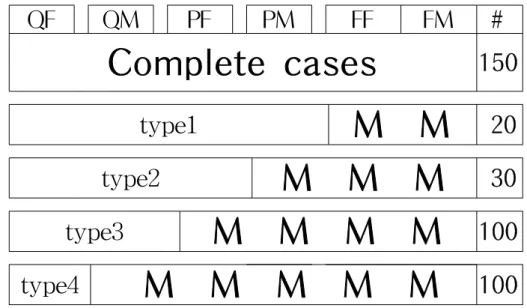
The monotone missing pattern in Figure 1 is considered. There are 150 complete cases and 4 missing types. In type1, 20 cases are missing on FF and FM. In type2, 30 cases are missing on PM, FF and FM. See Figure 1 for other types.
The capital letter `M' in Figure 1 indicates missing values.
MCAR and MAR missing mechanisms are considered simultaneously in one data set. From the generated random values, keep 170 cases from the top and then the rest 230 cases are sorted according to QF by ascending. The values located on the missing blocks are missing. Then the missing mechanism of type1 is `MCAR'.
Since the missingness for type2, type3, and type4 depends on the value of QF, the missing mechanism of these types are `MAR'. For example, the units have much larger values on QF tend to have missing type4.
Data sets are generated 1000 times and 400 cases are generated per each data set. For each data set, the covariance matrices are estimated by EM algorithm and Multiple Imputation(MI) methods. We calculate average and variance of 1000 estimates for each element of the covariance matrix. Two methods are compared
to check biases and efficiency for the estimates of variances-covariance matrix.
QF QM PF PM FF FM #
Complete cases
150type1
M M
20type2
M M M
30type3
M M M M
100type4
M M M M M
100Figure 1: Monotone missing pattern considered in this study
4. Simulation Results
Complete-case analysis(CC), available-case analysis(AC), EM algorithm, and multiple imputation(MI) methods are compared in this section. For multiple imputation, data augmentation(Tanner and Wong, 1987) was used to generate imputed data and construct 5 completed tables. Some S-PLUS 6.1(2001) functions for missing values were used to do MI and EM in this study.
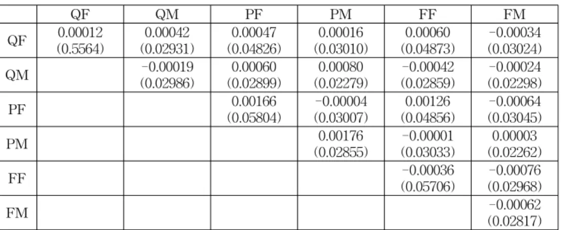
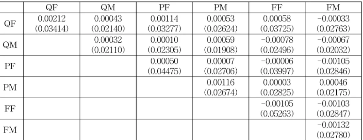
Table 1-4 have 5× 5 matrix forms and the numbers show the biases and standard errors(S.E.) of the corresponding elements of variances and covariances for 5 variables such as QM, PF, PM, FF, and FM. The values in parenthesis are S.E.'s and the other values are the biases. The biases in the tables are the average of 1000 biases from 1000 simulated data set. The bias is calculated as sample covariance matrix minus true covariance matrix for each completed data set by the corresponding method. The S.E's are the square root of sample variances of 1000 estimates of the corresponding elements of variances and covariances. Table 5 shows that sum of the 21 biases and S.E.'s in the corresponding tables and the values on MSE column are sum of 21 MSE which is calculated by (bias2 + variances of 1000 estimates).
If we are interested in the bias of point estimation, complete cases analysis(CC) is not bad. The performance of CC analysis is reliable if there are strong evidence
that the complete cases have enough information to represent the population. In this simulation study, there are 150 complete cases out of 400 cases in each data set. The 150 cases are enough to reveal the association between variables, but the variation of estimates is larger than the other methods. Many ways of multivariate analysis are based on the variance-covariance matrix without any testing like factor analysis. In this case, the variance-covariance matrix obtained from the complete cases analysis can be used.
The estimation of the association of QF, QM, and PF is seriously biased for the available analysis. The association of three variables are much distorted when we calculate variances and covariances based on the available cases because the missingness of QM and PF depends on the value of QF. If we can't ignore the MAR missingness, available case analysis can be the worst.
EM and MI can be generally more preferred than the traditional two methods.
Table 5 shows that EM algorithm has less MSE than other methods.
Table 1: Complete case analysis results
QF QM PF PM FF FM
QF 0.00012 (0.5564)
0.00042 (0.02931)
0.00047 (0.04826)
0.00016 (0.03010)
0.00060 (0.04873)
-0.00034 (0.03024)
QM -0.00019
(0.02986)
0.00060 (0.02899)
0.00080 (0.02279)
-0.00042 (0.02859)
-0.00024 (0.02298)
PF 0.00166
(0.05804)
-0.00004 (0.03007)
0.00126 (0.04856)
-0.00064 (0.03045)
PM 0.00176
(0.02855)
-0.00001 (0.03033)
0.00003 (0.02262)
FF -0.00036
(0.05706)
-0.00076 (0.02968)
FM -0.00062
(0.02817)
Table 2: Available case analysis results
QF QM PF PM FF FM
QF 0.00212 (0.03414)
-0.01452 (0.01914)
0.07372 (0.04613)
0.00033 (0.02784)
0.00060 (0.04873)
-0.00034 (0.03024)
QM -0.00344
(0.02061)
0.01560 (0.02650)
0.00066 (0.02104)
-0.00042 (0.02859)
-0.00024 (0.02298)
PF 0.05212
(0.05398)
0.00020 (0.02826)
0.00126 (0.04856)
-0.00064 (0.03045)
PM 0.00169
(0.02707)
-0.00001 (0.03033)
0.00003 (0.02262)
FF -0.00036
(0.05706)
-0.00076 (0.02968)
FM -0.00062
(0.02817)
Table 3: EM algorithm results
QF QM PF PM FF FM
QF 0.00212 (0.03414)
0.00043 (0.02140)
0.00114 (0.03277)
0.00053 (0.02624)
0.00058 (0.03725)
-0.00033 (0.02763)
QM 0.00032
(0.02110)
0.00010 (0.02305)
0.00059 (0.01908)
-0.00078 (0.02496)
-0.00067 (0.02032)
PF 0.00050
(0.04475)
0.00007 (0.02706)
-0.00006 (0.03997)
-0.00105 (0.02846)
PM 0.00116
(0.02674)
0.00003 (0.02825)
0.00046 (0.02175)
FF -0.00105
(0.05263)
-0.00103 (0.02847)
FM -0.00132
(0.02780)
Table 4: Multiple imputation results
QF QM PF PM FF FM
QF 0.00212 (0.03414)
0.00034 (0.02218)
0.00121 (0.03375)
0.00040 (0.02784)
0.00174 (0.03850)
0.00001 (0.02912)
QM 0.00117
(0.02181)
0.00037 (0.02453)
0.00148 (0.01988)
-0.00052 (0.02637)
0.00035 (0.02136)
PF 0.00530
(0.04710)
0.00057 (0.02901)
0.00327 (0.04180)
-0.00032 (0.03067)
PM 0.00626
(0.02835)
0.00062 (0.03024)
0.00178 (0.02327)
FF 0.00738
(0.05582)
-0.00023 (0.03065)
FM 0.00447
(0.02984)
Table 5: Summary of biases, S.E., and MSE
Method Bias S.E. MSE
CC 0.01151021 0.7390429 0.02882395
Avail 0.16967810 0.6821126 0.03335948
EM 0.01430794 0.6138044 0.01940924
MI 0.03992406 0.6462332 0.02164932
5. Discussion
Advantages of complete-case analysis are simplicity, since standard complete data statistical analyses can be applied without modifications, and comparability of univariate statistics, since these are all calculated on a common sample base of
cases. Disadvantages stem from the potential loss of information in discarding incomplete cases. This loss of information has two implications: loss of precision, and bias when the missing-data mechanism is not MCAR (ie., the complete cases are not a random sample of all the cases). We can expect better estimates of means and variances under MCAR, using the available-case analysis instead of complete-case analysis, but it is not true in general for covariances or correlations. Most people do these two methods when they have incomplete data for their simplicity. Neither method, however, is generally satisfactory.
The EM algorithm is a general approach for computing maximum likelihood estimates of parameters from incomplete data. The performances of EM algorithm and MI in monotone missing pattern are better than the tradition two methods.
EM algorithm and MI have less MSE than the traditional methods.
If we are interested in just point estimation, EM algorithm and some single imputation method like stochastic regression imputation method are quite satisfactory. Since the single imputation methods do not account for imputation uncertainty, a key problem for single imputation is that the standard errors computed from the filled-in data are underestimated. Replication methods like jackknife and multiple imputation(MI) have been developed to address this problem.
EM algorithm with jackknife method is a possible way to get a valid standard errors than other methods. Multiple imputation requires less computation than resampling methods. However, the MI variance estimator tends to be larger than the Jackknife variance estimator with EM algorithm.
References
1. Dempster, A. P., Laird, N. M. and Rubin, D. B. (1977). Maximum likelihood from incomplete data via the EM algorithm(with discussion).
Journal of the Royal Statistical Society Series B, 39, 1-38.
2. Little, R. J. A. and Rubin, D. B. (2002). Statistical analysis with missing data. J. Wiley & Sons, New York.
3. Rubin, D. B. (1976). Inference and missing data(with discussion).
Biometrika, 63, 581-592.
4. Rubin, D. B. (1978). Multiple Imputation in Sample Surveys - A Phenomenological Bayesian Approach to Nonresponse, Proceedings of the Survey Research Methods Section, American Statistical Association, 1978, 20-34
5. S-Plus 6.1 Manual (2001). Analyzing Data with Missing Values in S-Plus, Insightful Corporation. Seattle, Washington.
6. Tanner, M. A. and Wong, W. H. (1987). The calculation of posterior
distributions by data augmentation(with discussion). Journal of the American Statistical Association, 82, 528-550.
[ received date : Oct. 2004, accepted date : Dec. 2004 ]