Application of Deep Learning in Dentistry and Implantology

pISSN 1229-5418 eISSN 2671-6623

Implantology 2020; 24(3): 148-181 https://doi.org/10.32542/implantology.202015

Received: June 9, 2020 Revised: July 25, 2020 Accepted: July 29, 2020 ORCID

Dae-Young Kang

https://orcid.org/0000-0002-4311-4118 Hieu Pham Duong

https://orcid.org/0000-0001-5409-0361 Jung-Chul Park

https://orcid.org/0000-0002-2041-8047 Copyright © 2020. The Korean Academy of Oral &

Maxillofacial Implantology

This is an Open Access article distributed under the terms of the Creative Commons Attribution Non-Commercial License (http://creativecommons.

org/licenses/by-nc/4.0/) which permits unrestricted non-commercial use, distribution, and reproduction in any medium, provided the original work is properly cited.

OPEN ACCESS

Artificial intelligence and deep learning algorithms are infiltrating various fields of medicine and dentistry. The purpose of the current study was to review literatures applying deep learning algorithms to the dentistry and implantology. Electronic literature search through MEDLINE and IEEE Xplore library database was performed at 2019 October by combining free-text terms and entry terms associated with ‘dentistry’ and ‘deep learning’. The searched literature was screened by title/abstract level and full text level. Following data were extracted from the included studies:

information of author, publication year, the aim of the study, architecture of deep learning, input data, output data, and performance of the deep learning algorithm in the study. 340 studies were retrieved from the databases and 62 studies were included in the study. Deep learning algorithms were applied to tooth localization and numbering, detection of dental caries/periodontal disease/

periapical disease/oral cancerous lesion, localization of cephalometric landmarks, image quality enhancement, prediction and compensation of deformation error in additive manufacturing of prosthesis. Convolutional neural network was used for periapical radiograph, panoramic radiograph, or computed tomography in most of included studies. Deep learning algorithms are expected to help clinicians diagnose and make decisions by extracting dental data, detecting diseases and abnormal lesions, and improving image quality.

Keywords: Deep learning; Dentistry; Dental implants; Machine learning; Neural networks;

Radiography, Dental

Ⅰ. Introduction

The Go competition between the artificial intelligence (AI) AlphaGo of Google DeepMind and the legendary Go player Lee Sedol-in which AlphaGo won 4:1- straightforwardly shows the development of AI. At present, AI is being widely used in

Abstract

* Corresponding author: Jung-Chul Park, Professor, Department of Periodontology, Dankook University College of Dentistry, 119 Dandae-ro, Dongnam-gu, Cheonan 31116, Korea.

Tel: +82-41-550-1931. Fax: +82-303-3442-7364. E-mail: [email protected]

Implantology

Dae-Young Kang, DDS, MSD

, Hieu Pham Duong, DDS, MSD, PhD

, Jung-Chul Park, DDS, MSD, PhD

1 Clinical Assistant Professor, Department of Periodontology, Dankook University College of Dentistry, Cheonan, Korea

2 Associate Dean, Department of Maxillo-Stomatology, Vietnam National University School of Medicine and Pharmacy, Hanoi, Vietnam

3Associate Professor, Department of Periodontology, Dankook University College of Dentistry, Cheonan, Korea

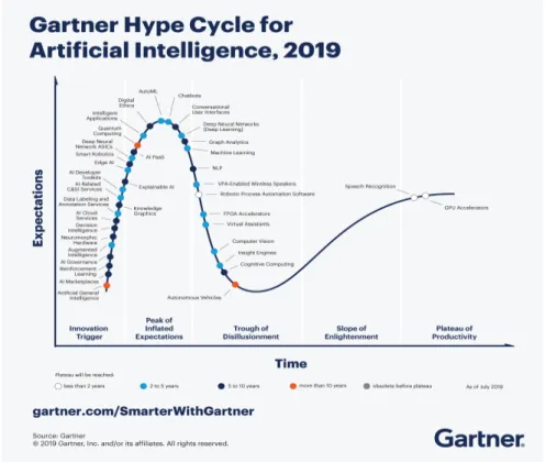
various fields including SPAM mail filters, search algorithms and ranking system of web search engines, facial recognition algorithms of social networking services, and personalized curation algorithms of contents or products (Fig. 1).

Alibaba achieved daily sales $38 billion during the Singles Day in 2019, 26% higher than the previous year, by launching an AI fashion assistant which has been trained about hundreds of millions of clothes. Amazon is automating most of their logistics except packing and is managing “Amazon Go” checkout-free convenience store chain in the US. In the Amazon Go, the payment is automatically processed when customers exit with their products based on real-time location tracking of them using multiple cameras, weight measuring sensors, and deep learning algorithms.

AI is expected to have huge impact on the healthcare industry. Currently, more than 40 and 10 deep learning algorithms have been approved as medical devices by the US Food and Drug Administration (FDA) and Ministry of Food and Drug Safety (MFDS) in South Korea, respectively. For example, fourth-generation Apple Watch and AliveCor KardiaMobile with deep learning algorithm have been approved by the US FDA as over-the-counter medical devices for detecting atrial fibrillation. These algorithms show an accuracy for detecting abnormal findings comparable to that of humans by training hundreds of thousands of data.

Fig. 1. Hype cycle for artificial intelligence 2019. Reprinted from “Gartner Hype Cycle for Artificial

Intelligence 2019” by Kenneth Brant, Jim Hare, Svetlana Sicular, Copyright 2019 by Gartner, Inc. and/or

its affiliates. https://www.gartner.com/smarterwithgartner/top-trends-on-the-gartner-hype-cycle-for-

artificial-intelligence-2019/

Dentistry is a field of study that requires a high level of accuracy; it is expected that AI and deep learning algorithms will be introduced in the near future and provide great assistance to clinical practices.

In South Korea, an algorithm that estimates bone age from a hand-wrist radiograph has been approved by the MFDS; however, not many other cases have been reported yet. Therefore, this study aims to examine the global trends of deep learning technologies applied to dentistry and to forecast the future of dentistry.

Ⅱ. Materials and Methods

1. Literature Search

To select literature on the application of deep learning algorithms in dentistry, we searched the MEDLINE and IEEE Xplore databases for papers in all languages that were published before October 24, 2019. The search formula was set up by combining free-text term and entry term about the deep learning, neural network, and dentistry (Table 1).

2. Selection of Papers

Papers were selected in two steps: first, papers were selected based on their title and abstract; second, their full text was evaluated. The criteria for selecting papers were as follows: (1) papers for clinical

MEDLINE

1. “Deep learning” [tiab] OR “Neural network” [tiab] OR “Neural networks” [tiab] OR “Neural Net” [tiab] OR

“Neural Nets” [tiab]

2. “Neural Networks (computer)” [Mesh]

3. 1 OR 2

4. “Dental” [tiab] OR “Dentistry” [tiab]

5. “Dentistry” [mesh] OR “Radiography, Dental” [mesh] OR “Dental implants” [mesh] OR “Stomatognathic Diseases” [mesh] NOT “Pharyngeal Diseases” [mesh]

6. 4 OR 5 7. 3 AND 6 IEEE Xplore database

1. “All Metadata” : Deep learning OR “All Metadata” : Neural Network OR “All Metadata” : Neural Networks OR

“All Metadata” : Neural Net OR “All Metadata” : Neural Nets 2. “Mesh_Terms” : Neural networks (computer)

3. 1 OR 2

4. “All Metadata” : Dental OR “All Metadata” : Dentistry

5. “Mesh_Terms” : Dentistry OR “Mesh_Terms” : Radiography, dental OR “Mesh_Terms” : Dental implants OR

“Mesh_Terms” : Stomatognathic Diseases NOT “Mesh_Terms” : Pharyngeal Diseases 6. 4 OR 5

7. 3 AND 6

Table 1. Search strategy

purpose rather than data mining or statistical analysis and (2) papers based on studies using deep neural networks such as convolution neural networks (CNNs), recurrent neural networks (RNNs), or generative adversarial networks (GANs), rather than machine learning among the AI fields.

3. Data Extraction

From the selected studies, we extracted information of the authors, publication years, deep learning architectures that were used, input data, output data, and performance metrics of the algorithm. We examine these data in detail below.

1) Deep learning architectures (1) CNNs

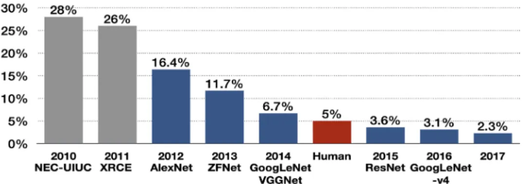
CNNs attracted attention after they won the ImageNet Challenge from 2012–2017, which is a large- scale image recognition contest for classifying 50,000 high-resolution color images into 1,000 categories after training 1.2 million images, held every year since 2010 (Fig. 2). In 2012, AlexNet

decreased the top-5 error rate by 10% to 16.4%, and SENet achieved 2.3% in 2017.

The origin of the CNN is the Neocognitron Model,

which applied a neurophysiological theory to an artificial neural network based on the principle that only certain neurons in the visual cortex are activated according to the shape of target object.

CNNs largely comprise three layers: convolutional layer, pooling layer, and fully connected layer. The convolutional layer creates a feature map by arranging the outputs of convolution operation at each position of square filter while the filter is sliding over the input

Fig. 2. Algorithms that won the ImageNet Large Scale Visual Recognition Challenge (ILSVRC) in 2010–

2017. The top-5 error refers to the probability that all top-5 classifications proposed by the algorithm

for the image are wrong. The algorithms with blue graph are convolutional neural network. Although

VGGNet took second place in 2014, it is widely used in studies as its concise structure. Adapted from “A

fully-automated deep learning pipeline for cervical cancer classification” by Alyafeai Z., Ghouti L., Expert

Systems with Applications Proceedings of the IEEE 2019;141;112951. Copyright 2019 by Elsevier Ltd.

data. It has the advantage of preserving horizontal and vertical information among pixels compared to the fully connected neural network, which converts images to one-dimensional vector. The pooling layer downsamples size of the feature map and summarizes important information in the feature map; the classification value is then output through the fully connected layer. For example, LeNet, which was the first CNN that classified hand-written numbers with an error rate of 0.95%, comprises three convolutional layers, three pooling layers, and one fully connected layer (Fig. 3).

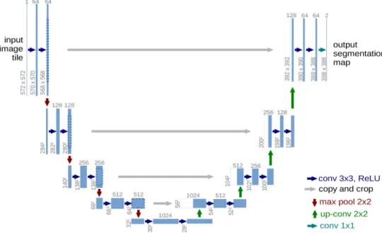
Meanwhile, U-Net, which is used for region segmentation of medical images, does not have a fully connected layer. It comprises an encoder part, which extracts a feature map by convolution and pooling, and a decoder part, which restores the segmented images from the feature map by “up-convolution”

(Fig. 4).

Fig. 4. Architecture of U-net. Reprinted from “U-net: Convolutional networks for biomedical image segmentation” by Ronneberger O., Fischer P., Bottou L, Brox T., Lecture Notes in Computer Science 2015;9351:234-241. Copyright 2015 by Elsevier Ltd.

Fig. 3. Architecture of LeNet-5. Reprinted from “Gradient-based learning applied to document recognition” by LeCun Y., Bottou L, Bengio Y. et al., Proceedings of the IEEE 1998;86;2278–2323.

Copyright 1998 by IEEE.

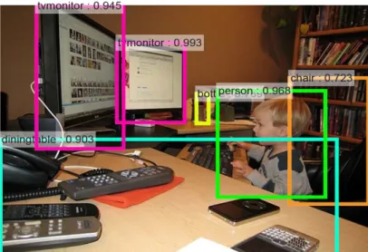
When detecting multiple objects in a single image, a region-based CNN (R-CNN) is used, which includes a region proposal network for the recognition of objects and their positions (Fig. 5).

The region proposal network suggests anchor boxes of various ratios and sizes for the input image, and those that have a high intersection-over-union (IOU) with the previously trained images are selected.

(2) RNNs

RNNs can analyze time-series data that are arranged in chronological sequence such as voice signals.

Therefore, they are utilized to predict indices such as stocks, for voice recognition, text translation, adding image captions, and image or music generation. A video of former US president Barack Obama appearing to give a speech has been published, in which the algorithm synthesize lip motion synchronized with his original voice.

This neural network receives the input values from not only the previous layer ( X

) but also the recurrent neurons of the previous time step, transforms, and delivers them to the next layer and recurrent neurons of the next time step, unlike the feed-forward neural network that only delivers signals from the input layer to the output layer (Fig. 6).

Fig. 5. Multiple object recognition in region-based convolutional neural network. Reprinted from

“Faster R-CNN: Towards Real-Time Object Detection with Region Proposal Networks” by Ren S., He, K., Girshick, R., Sun, J., IEEE Transactions on Pattern Analysis and Machine intelligence 2017;39(6):1137–

1149.

Fig. 6. Structure of recurrent neural network. Right illustrates unfold structure from left to right over

time. Reprinted from http://colah.github.io/posts/2015-08-Understanding-LSTMs/

When an RNN—in a pure sense (also referred to as a “vanilla RNN”)—with the above characteristics is configured with deep layers, there are problems such as gradient vanishing/exploding and the long- term dependency. To solve these problems, changes in connections among cells (the units of neural networks) including skip connection or leaky units, long short-term memory cells,

and gated recurrent unit cells

using gates inside the cells have been proposed.

(3) GANs

GANs are unsupervised learning algorithms,

which have a neural network generating an answer inside a neural network (the generator) competes with a neural network that evaluates it (the discriminator).

The fake answers proposed by the generator are gradually similar to the ground truth with the aid of the feedback from the discriminator.

2) Output data of deep learning

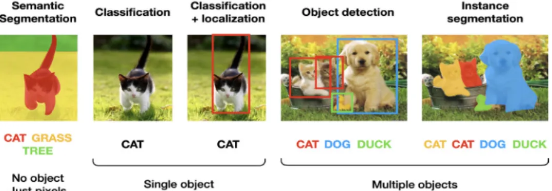
The results of deep learning image analysis can be largely divided into five types as follows (Fig. 7).

(1) Classification: The objects in image are classified as the most likely option to be ground truth among predetermined options. One example is LeNet-5, which classified hand-written numbers into 10 types, from 0 to 9. (2) Object localization: This is to indicate the locations of objects in image by bounding boxes. When object localization and classification are performed simultaneously, it is called object detection. (3) Semantic segmentation: This means to segment whole image according to the pixel-based classification without object recognition. (4) Instance segmentation: This recognizes each object and delineates its outline in an image. (5) Image reconstruction: Examples include image quality enhancement by super-resolution or artifact reduction, and class activation maps overlap heat map, which changes the color depending on the contribution of the classification, to the input image. This allows visual confirmation based on which areas of the image are classified using the deep learning algorithm.

Fig. 7. Computer vision tasks. Adapted from “https://www.slideshare.net/darian_f/introduction-to-the-

artificial-intelligence-and-computer-vision-revolution.”

3) Performance metrics of deep learning algorithms

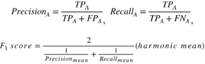
The representative performance metrics for classification algorithms are accuracy, precision, recall, F1 score, and the area under the receiver operating characteristic curve (AUC). Other metrics except AUC can be calculated using the confusion matrix illustrating whether the predicted classification matches the ground truth (Fig. 8).

For example, when we evaluate the accuracy of a deep learning model that classifies images into three types, we can calculate the accuracy simply by dividing the number of cases which classify A as A, B as B, or C as C by the total number of cases.

( TP=True Positive, FP=False Positive, TN=True Negative, FN=False Negative )

Furthermore, the F

score can be calculated by determining the precisions ( Precision

, Precision

, and Precision

) and recalls ( Recall

, Recall

, and Recall

) for classifying A, B, and C, and calculating the mean precision ( Precision

) and mean recall ( Recall

), and then calculating the harmonic mean of these two.

The evaluation indices for object localization and segmentation include the IOU and the dice similarity coefficient, in addition to the above-mentioned indices (Fig. 9). IOU is also called Jaccard index and is calculated by dividing the overlapping area between the ground truth and the predicted areas by the union area. The dice similarity coefficient is calculated by dividing the double of the overlapping area by the sum of each area.

Fig. 8. Confusion matrix to calculate accuracy (A) and to calculate precision recall, and F

score (B).

Ⅲ. Results

1. Literature Search and Selection of Studies

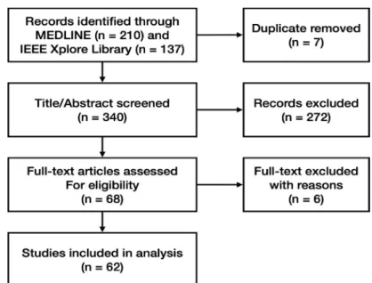
We found 340 papers by searching MEDLINE and the IEEE Xplore Library, excluding 7 duplicates.

After evaluating the titles and abstracts, we excluded 272 papers and evaluated the full texts of 68 papers.

A total of 62 papers were included in the study (Fig. 10). The excluded papers and the reasons for their exclusion are outlined in Suppl. 1.

Fig. 9. Evaluation of object localization (A) and object segmentation (B).

Fig. 10. Flow chart showing literature search and selection.

2. Data Extraction

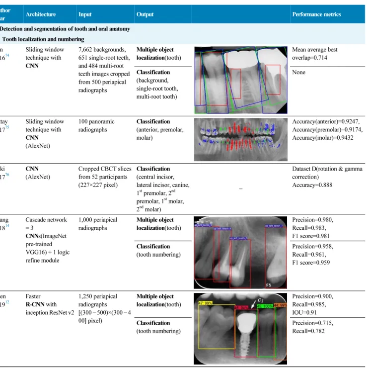
The characteristics of the selected studies and the extracted data are listed in Table 2.

Table 2. Characteristics of included studies.

Author Year

Architecture Input Output Performance metrics

1. Detection and segmentation of tooth and oral anatomy 1.1 Tooth localization and numbering

Eun 2016

74

Sliding window technique with CNN

7,662 backgrounds, 651 single-root teeth, and 484 multi-root teeth images cropped from 500 periapical radiographs

Multiple object localization(tooth)

Mean average best overlap=0.714 Classification

(background, single-root tooth, multi-root tooth)

None

Oktay 2017

75

Sliding window technique with CNN (AlexNet)

100 panoramic radiographs

Classification (anterior, premolar, molar)

Accuracy(anterior)=0.9247, Accuracy(premolar)=0.9174, Accuracy(molar)=0.9432

Miki 2017

76

CNN (AlexNet)

Cropped CBCT slices from 52 participants (227×227 pixel)

Classification (central incisor, lateral incisor, canine, 1

premolar, 2

premolar, 1

st

molar, 2

nd

molar)

–

Dataset D(rotation & gamma correction)

Accuracy=0.888

Zhang 2018

14

Cascade network

= 3

CNNs(ImageNet pre-trained VGG16) + 1 logic refine module

1,000 periapical radiographs

Multiple object localization(tooth)

Precision=0.980, Recall=0.983, F1 score=0.981 Classification

(tooth numbering)

Precision=0.958, Recall=0.961, F1 score=0.959

Chen 2019

12

Faster R-CNN with inception ResNet v2

1,250 periapical radiographs [(300–500)×(300–4 00] pixel)

Multiple object localization(tooth)

Precision=0.900, Recall=0.985, IOU=0.91 Classification

(tooth numbering)

Precision=0.715, Recall=0.782

Table 2. Characteristics of included studies

Tuzoff 2019

13

Faster R-CNN with VGG16

1,574 panoramic radiographs

Multiple object localization(tooth)

Precision=0.9945, Recall

†

=0.9941 Classification

(tooth numbering)

Specificity=0.9994, Recall

†

=0.9800

Expert Multiple object

localization(tooth)

Precision=0.9998, Recall

†

=0.9980 Classification

(tooth numbering)

Specificity=0.9997, Recall

†

=0.9893 Koch

2019

77

6 modifications of U-Net

1,500 panoramic radiographs

Classification(1–4:

32, teeth with/without restoration and with/without orthodontic appliance, 5: implant, 6: >32 teeth , 7–10:

<32 teeth with/without restoration and with/without orthodontic appliance)

Ensemble of U-Net modification 1 and 4 Accuracy=0.952, Precision=0.933, Recall

†

=0.944, Specificity=0.961, DSC=0.936

Mask R-CNN Accuracy=0.98,

Precision=0.94, Recall

†

=0.84,

Specificity=0.99, DSC=0.88 Hiraiwa

2019

78

CNN(AlexNet) 760 cropped images of mandibular 1

st

molar from 400 panoramic radiographs CBCT images from 400 participants (ground truth)

Prediction(number of distal root of mandibular 1

st

molar)

Accuracy=0.874, Recall

†

=0.773, Specificity=0.971, Precision

=0.963, NPV=0.818, AUC=0.87, Training time=51 minutes, Testing time=9 seconds

CNN(GoogleNet) Accuracy=0.853,

Recall

†

=0.742, Specificity=0.959, Precision

=0.947, NPV=0.800, AUC=0.85, Training time=3 hours, Testing time=11 seconds

Expert radiologist Accuracy=0.812,

Recall

†

=0.802, Specificity=0.820 Precision

†

=0.787, NPV=0.834, AUC=0.74 1.2. Tooth segmentation

Jader 2018

15

Mask R-CNN with ResNet101

1,500 panoramic radiographs

Instance segmentation

None

Classification(1–4:

32, teeth with/without restoration and with/without orthodontic appliance, 5: implant, 6: >32 teeth , 7–10:

<32 teeth with/without restoration and with/without orthodontic appliance)

Accuracy=0.98,

Precision=0.94,

Recall=0.84,

F1 score=0.88,

Specificity=0.99

Vinaya- halingam 2019

79

CNN(U-Net) 81 panoramic radiographs

Instance segmentation (3

rd

molar)

DSC=0.936, IOU=0.881, Recall

†

=0.947, Specificity=0.999 Segmentation

(mandibular canal)

DSC=0.805, IOU=0.687, Recall

=0.847, Specificity=0.967 De Tobel

2017

21

CNN(ImageNet pre-trained AlexNet)

20 cropped images of lower left 3

rd

molar (240×390 pixel) from 20 panoramic radiographs

Classification (modified Demirjian’s staging, 0–9)

Mean accuracy=0.51, Mean absolute difference=0.6 stages

Merdietio 2019

16

CNN(AlexNet) 400 panoramic radiographs

Segmentation (lower left 3

rd

molar)

Accuracy=0.61

Classification (Modified Demirjian’s staging, 0–9)

Accuracy=0.61 Mean absolute difference=0.53 stages Cohen’s 

=0.84

Tian 2019

17

CNN(sparse octree structure, voxel-based)

3D scanned images of 600 dental models

Classification (tooth numbering)

Recall

†

=0.9800, Specificity=0.9994 Instance

segmentation(tooth)

Accuracy=0.8981

Expert Classification

(tooth numbering)

Recall

†

=0.9893, Specificity=0.9997

Xu 2019

18

CNN 3D scanned mesh

images from 1,200 dental models

Instance segmentation (tooth–gingiva, tooth–tooth)

Accuracy(maxilla)=0.9906 Accuracy(mandible)=0.9879

1.3. Bone segmentation Duong

2019

20

CNN(U-Net) 50 intraoral ultrasonic images on 8 lower incisors from piglets (128×128 pixel)

Segmentation (alveolar bone)

DSC=75.0±12.7%,

Recall

=77.8±13.2%,

Specificity=99.4±0.8%

Minnema 2019

19

CNN(MS-D Net) CBCT from 20 patients

Segmentation(bone) DSC=0.87±0.06,

Mean absolute deviation=0.44 mm

CNN(U-Net) DSC=0.87±0.07,

Mean absolute deviation=0.43 mm

CNN(ResNet) DSC=0.86±0.05,

Mean absolute deviation=0.40 mm Snake evolution

algorithm

DSC=0.78±0.07, Mean absolute deviation=0.57 mm 2. Image quality enhancement

Du 2018

22

CNN Center-cropped

images from 5,166 panoramic radiographs

(256×256 or 384×384 pixel)

Image reconstruction (compensating blurring from the positioning error)

Model 1

Mean standard error=0.339, Mean absolute error=0.749, Maximum absolute error=1.499

Liang 2018

23

Hanning + filtered back projection

CBCT from 3,872 patients

Image reconstruction (noise and artifact reduction)

Root mean square error=0.1180, SSI=0.9670

Non-local mean weighted least square iterative reconstruction

Root mean square error

=0.0862, SSI=0.9839

Network reconstruction

Root mean square error

=0.1015, SSI=0.9800

Hu 2019

24

GAN Low-dose CBCT

images from 44 patients

Image reconstruction (noise and artifact reduction)

PSNR(360°)=32.657, SSI(360°)=0.925,

Noise suppression=5.52±0.25, Artifact correction=6.98±0.35, Detail restoration=5.56±0.31, Comprehensive

quality=6.52±0.34, Training time per batch=0.691,

Testing time per batch=0.183

CNN (180 180°scanned

images, 120 360°

scanned images)

PSNR(360°)=34.402, SSI(360°)=0.934,

Noise suppression=8.95±0.36, Artifact correction=7.20±0.23, Detail restoration=5.35±0.28, Comprehensive

quality=7.54±0.32, Training time per batch=0.726,

Testing time per batch=0.183

m-WGAN Normal dose CBCT

images (ground truth)

PSNR(360°)=33.824, SSI(360°)=0.975,

Noise suppression=8.20±0.35, Artifact correction=7.46±0.27, Detail restoration=8.98±0.20, Comprehensive

quality=8.25±0.21, Training time per batch=0.798,

Testing time per batch=0.184 Hegazy

2019

25

CNN(U-Net) 1,000 projection images (0–180°) from 5 patients who had different kinds of metal implants and dental fillings at different tooth positions

Segmentation (metal)

Mean IOU=0.94 Mean DSC=0.96

Image reconstruction (metal artifact reduction)

Mean relative error=94.25%

Mean normalized absolute difference=93.25%

Mean sum of square difference=91.83%

Conventional segmentation method

Original CBCT images

Segmentation (metal)

Mean IOU=0.75 Mean DSC=0.86

Image reconstruction (metal artifact reduction)

Mean relative error=91.71%

Mean normalized absolute difference=95.06%

Mean sum of square

difference=93.64%

Dinkla 2019

26

CNN(U-Net) 3D patch (48×48×48 voxel) from 34 head and neck T2-weighted MRI

CT(ground truth)

Image reconstruction (synthetic computed tomography)

Comparing synthetic CT and conventional CT, Mean DSC=0.98±0.01, Mean absolute error=75±9 HU

Mean error=9±11 HU, Mean voxel-wise dose differences=–0.07±0.22%, Mean gamma pass rate=95.6±2.9%.

Mean dose

difference=0.0±0.6%(body volume),

–0.36±2.3%(high-dose volume)

Hatvani 2019

27

CBCT(original) CBCT of 13 teeth (linewidth resolution=500µm, voxel size

=80×80×80µm

3

), Micro-CT of 13 teeth (linewidth

resolution=50µm, voxel

size=40×40×40µm

3

) (ground truth)

Image reconstruction (super-resolution) DSC=0.88

Mean of difference - Feret=176, Mean of difference - Area=0.1139

LRTV DSC=0.89, Time=6988

(maxillary anterior teeth), 9059(mandibular premolar), 10301 seconds(mandibular molar), Mean of difference - Feret=113, Mean of difference - Area =0.1395

TF-SISR DSC=0.90,

Time=71(maxillary anterior teeth), 92(mandibular premolar), 104 seconds (mandibular molar), Mean of difference - Feret=95, Mean of difference - Area=0.0987 Hatvani

2019

28

CBCT(original) 5,680 CBCT slices of 13 teeth

5,680 micro-CT slices of 13 teeth

(ground truth)

Image reconstruction (super-resolution) DSC=0.8891,

Difference of the endodontic volumes

(CBCT– µCT)=12.39%

SRR:l

DSC=0.8852

Difference of the endodontic volumes

(SRR:l

– µCT)=12.25%

SRR:TV DSC=0.8913

Difference of the endodontic volumes

(SRR:l

– µCT)=12.40%

CNN (U-Net)

DSC=0.8998

Difference of the endodontic volumes

(U-net– µCT)=10.12%

CNN

(Subpixel network)

DSC=0.9101

Difference of the endodontic volumes(Subpixel network–

µCT)=6.07%

3. Disease detection 3.1. Detection of dental caries Kumar

2018

29

CNN(U-Net) >6,000 bitewing radiographs

Instance segmentation (dental caries)

Recall=0.70, Precision=0.53, F1 score=0.603

CNN(U-Net) + incremental example mining

Recall=0.73, Precision=0.53, F1 score=0.614

CNN(U-Net) + hard example mining

Recall=0.69, Precision=0.46, F1 score=0.552

Lee 2019

30

CNN (ImageNet pre-trained GoogleNet Inception v3)

3,000 periapical radiographs

Classification (caries, non-caries)

–

Accuracy=82.0, Recall

=81.0, Specificity=83.0, Precision

†

=82.7, NPV=81.4 in premolar and molar area Casalegno

2019

31

CNN

(encoding path of U-Net replaced with the ImageNet Pre-trained VGG16)

217 near-infrared transillumination images (256×320 pixel)

Semantic segmentation (background, enamel, dentin, proximal caries, occlusal caries

Mean IOU=0.727,

IOU(proximal caries)=0.495, IOU(occlusal caries)=0.490, AUC(proximal caries)=0.856, AUC(occlusal caries)=0.836

Moutselos 2019

32

Mask R-CNN with ResNet101

79 clinical photos of occlusal surface

Classification in superpixel level

(international caries detection and assessment system 0: sound tooth surface,

1: first visual change in enamel, 2: distinct visual change in enamel, 3: localized enamel breakdown, 4: underlying dark shadow from dentin, 5: distinct cavity with visible dentine, 6: extensive distinct cavity with visible dentin)

F1 score(mc)=0.596, F1 score(cpc)=0.625, F1 score(wc)=0.684 3 indexes for the reduction back to superpixels(mc: most common, cpc: centroid pixel class, wc: worst class)

Classification in whole image level F1 score(mc)=0.889, F1 score (cpc)=0.778, F1 score (wc)=0.667

Liu 2019

34

Mask R-CNN with ResNet

12,600 clinical photos(1 mega pixel)

Multiple object localization, classification (dental caries, dental fluorosis,

periodontitis crack tooth, dental plaque, dental calculus, tooth loss)

Accuracy: 0.875(tooth

fluorosis)–1(tooth loss),

increase of the number of

treated patients by 18.4%,

mean diagnosis time reduces

by 37.5% for each patient

3.2. Detection of dental plaque and periodontal disease Yauney

2017

80

CNN

(truncated version of VGG16)

47(CD database) and 49(RD database) pairs of white light mode

Semantic segmentation (plaque, non-plaque)

Accuracy=0.8718, AUC=0.8720

and plaque mode intraoral photo (512×384 pixel) Bezruk

2017

35

CNN Malondialdehyde

concentration, Gluthatione concentration, Sulcus bleeding index

Classification (normal, gingivitis)

–

Precision=0.80, Recall=0.78, F1 score=0.78

Aberin 2018

36

CNN(AlexNet) 1,000 grayscale images with 600 magnification (227×227 pixel)

Classification (healthy, unhealthy)

Accuracy=0.76, Mean square error=0.05, Precision=0.68, Recall=0.98

Joo 2019

37

CNN 1,843 clinical photos of periodontal tissue

Classification (healthy periodontal status, mild periodontitis, severe periodontitis, not periodontal image)

–

Accuracy(healthy)=0.83, Accuracy(mild periodontitis)=0.74, Accuracy(severe periodontitis)=0.70, Accuracy(not periodontal image)=0.94

Krois 2019

38

CNN 2,001 cropped

panoramic radiographs

Classification (<20% bone loss,

≥20% bone loss)

–

Accuracy=0.81, Precision

†

=0.76, Recall

†

=0.81,

Specificity=0.81, NPV=0.85, AUC=0.89, F1 score=0.78

Dentist Accuracy=0.76,

Precision

†

=0.68, Recall

†

=0.92,

Specificity=0.63, NPV=0.90, AUC=0.77, F1 score=0.78 3.3. Detection of periapical diseases

Prajapati 2017

33

CNN

(2012 ImageNet pre-trained VGG16)

251 periapical radiographs (500×748 pixel)

Classification (dental caries, periapical infection, periodontitis)

–

Accuracy=0.8846

Ekert 2019

44

CNN 1,331 cropped

panoramic radiographs of 85 patients (64×64 pixel)

Classification (no attachment loss, widened periodontal ligament, clearly detectable lesion)

Recall

=0.74±0.19, Specificity=0.94±0.04 Precision

†

=0.67±0.14, NPV=0.95±0.04 AUC=0.95±0.02 In all teeth, majority(6) reference test condition Yang

2018

82

CNN(GoogLeNet Inception v3)

196 pairs of periapical radiograph before and after the treatments (96×192 pixel)

Classification (getting better, getting worse, have no explicit change)

Precision=0.537, Recall=0.490, F1 score=0.517

3.4. Detection of (pre)cancerous lesion Uthoff

2008

39

CNN 170 pairs of

Autofluorescence image and white light image

Classification (cancerous and pre-cancerous lesion, not suspicious)

Precision

=0.8767, Recall

†

=0.8500, Specificity=0.8875, NPV=0.8549, AUC=0.908;

Remote specialist Precision

=0.9494,

Recall

†

=0.9259, Specificity=0.8667, NPV=0.8125 Aubreville

2017

40

CNN

+Probability fusion

165,774 patches extracted from 7,894 grayscale confocal laser endomicroscopy video frames of the inner lower labium, the upper alveolar ridge, the hard palate (80×80 pixel)

Classification (normal, cancerous)

Accuracy=0.883, Recall

†

=0.866, Specificity=0.900, AUC=0.955

Forslid 2017

41

CNN

(VGG16, ResNet18)

Oral dataset 1 (15 microscopic cell images taken at ×20 magnification)

Classification (healthy, tumor)

VGG16 ResNet18

Accuracy=80.66±3.00, Precision=75.04±7.68, Recall=80.68±3.05, F1 score=77.68±5.28

Accuracy=78.34±2.37, Precision=72.48±4.46, Recall=79.00±3.37, F1 score 75.51±3.17 Oral dataset 2

(15 microscopic cell images taken at ×20 magnification)

Accuracy=80.83±2.55, Precision=82.41±2.55, Recall=79.79±3.75, F1 score=81.07±3.17

Accuracy=82.39±2.05, Precision=82.45±2.38, Rcall=82.58±1.92, F1 score 82.51±2.15 CerviSCAN dataset

(12,043 microscopic cell images taken at

×40 magnification)

Accuracy=84.20±0.86, Precision=84.35±0.97, Recall=84.20±0.86, F1 score=84.28±0.91

Accuracy=84.45±0.46, Precision=84.64±0.38, Rcall=84.45±0.47, F1 score 84.28±0.91 Herlev dataset

(917 microscopic cell images)

Accuracy=86.56±3.18, Precision=85.94±6.98, Recall=79.04±3.81, F1 score=82.16±3.85

Accuracy=86.45±3.81,

Precision=82.45±5.11,

Recall=84.45±2.16,

F1 score 83.36±3.65

Das 2018

42

CNN 1,000,000 patches

from 80 microscopic images taken at ×50 magnification (2,048×1,536 pixel)

Semantic segmentation (keratin, epithelial, subepithelial,

background)

Accuracy(epithelial)=0.984, Recall†(epithelial)=0.978, IOU(epithelial)=0.906, DSC(epithelial)=0.950, Accuracy(keratin)=0.981, IOU(keratin)=0.780, DSC(keratin)=0.752

Multiple object localization (keratin pearl)

Accuracy=0.969

Jeyaraj 2019

43

SVM 1,300 image patches

from 3 databases (BioGPS data portal=100, TCIA Archive=500, GDC Dataset=700)

Classification (normal, benign tumor, cancerous malignant)

–

Accuracy=0.82, Specificity=0.86, Recall

†

=0.76, AUC=0.725

DBN Accuracy=0.85,

Specificity=0.89, Recall

†

=0.82, AUC=0.85

CNN Accuracy=0.91,

Specificity=0.94, Recall

†

=0.91, AUC=0.965 Song

2019

83

Central attention residual network in CNN

48 tissue microarray core images (3,300×3,300 pixel)

Classification (tumor, stroma)

F1 score(RGB)=86.31%

DSC(RGB)=82.16%

3.5. Detection of other disease Murata

2019

45

CNN(AlexNet) 800 cropped panoramic radiographs of maxillary sinus (200×200 pixel)

Classification (healthy, inflamed)

Accuracy=0.875, Recall

†

=0.867, Specificity=0.883, Precision

=0.881, NPV=0.869, AUC=0.875

Radiologist Accuracy=0.896,

Recall

†

=0.900, Specificity=0.892, Precision

†

=0.893, NPV=0.899, AUC=0.896

Dental residents Accuracy=0.767,

Recall

=0.783, Specificity=0.750, Precision

†

=0.758, NPV=0.776, AUC=0.767 De Dumast

2018

46

NN 293 condyle images

from reconstructed CBCT

Classification(close to normal[control], close to normal [osteoarthritis], degeneration 1,2,3,4–5)

In confusion matrix, Accuracy=0.441,

Accuracy(including adjacent

1 cell around true positive

cell)=0.912

Kise 2019

47

CNN(AlexNet) 500 cropped CT images of parotid gland in 25 patients

Classification (normal, Sjögren syndrome)

Accuracy=0.96, Recall

=1, Specificity=0.92, AUC=0.960 Experienced

radiologist

Accuracy=0.983, Recall

=0.993, Specificity=0.779, AUC=0.996 Inexperienced

radiologist

Accuracy=0.835, Recall

=0.779, Specificity=0.892, AUC=0.997 Chu

2018

48

Octuplet Siamese network with 2-stage fine tuning

864 cropped panoramic radiographs (50×50 pixel)

Classification (normal, osteoporosis)

Accuracy=0.898

Kats 2019

49

Faster R-CNN (ResNet101)

65 panoramic radiographs

Multiple object localization (atherosclerotic carotid plaques)

Accuracy=0.83, Recall

=0.75

Specificity=0.80, AUC=0.83

4. Evaluation of facial esthetics, detection of cephalometric landmarks Murata

2017

50

CNN (ImageNet pre-trained VGG19) + LSTM

352 patients’ images (304×224 pixel)

Classification (mouth, jaw, face)

Accuracy=0.648

Mouth/left Jaw/left Face/remarkably distortion

Multiple CNNs Accuracy=0.630

Patcas 2019

51

CNN

(Internet Movie database-Wikipedia pre-trained, APPA-REAL and Chicago Face Dataset fine-tuned VGG16)

2,164 facial images of pre-/post-operation (Le Fort I osteotomy, sagittal split ramus osteotomy of the mandible, chin osteotomy, other osteotomies, 600 dpi)

Prediction apparent age, facial attractiveness (0 –100, 0: extremely unattractive, 100:

extremely attractive)

Mean difference between apparent age and actual age (pre-operation)=1.75 years Mean difference between apparent age and actual age (post-operation)=0.82 years Facial attractiveness was increased at 74.7% of patients

Leonardi 2010

52

Cellular NN (unsupervised learning)

40 lateral cephalometric radiographs, 22 landmarks

Image reconstruction (emboss

enhancement)

Euclidean distance mean

errors: higher for the

embossed images than for the

unfiltered radiographs

Accuracy of the

cephalometric landmark

detection improved on the

embossed radiograph but

only for a few points, without

statistical significance

Qian 2019

53

Faster R-CNN with VOC 2012 pre-trained ResNet50)

400 lateral cephalometric radiographs

Multiple object localization (19 landmarks)

Accuracy(test 1)=0.825, Accuracy(test 2)=0.724 Landmark can be classified as a ‘accurate’ on only if the distance between a detected landmark and its ground truth is less than 2 mm.

Torosdagli 2019

54

CNN (U-Net, deep geodesic learning), LSTM

25,600 slices from 50 3D reconstruced CBCT

Segmentation (mandible)

DSC=0.9386, Hausdorff distance=5.47

Multiple object localization (landmarks on mandible)

Mean error(mm):

coronoid process(left)=0, coronoid

process(right)=0.45, condyle(left)=0.33, condyle(right)=0.07, menton=0.03, gnathion=0.49, pogonion=1.54, B-point=0.33, infradentale=0.52

5. Fabrication of prosthesis Shen

2019

84

CNN(U-Net) 77 single crown models

Prediction (deformation, translation, scaling down, rotation)

F1 score(deformation)=0.9614, F1 score(scaling down)=0.9408, F1 score(translation)=0.9386, F1 score(rotation)=0.9387 Image reconstruction

(compensating deformation, translation, scaling down, rotation)

F1 score(deformation)=0.9699, F1 score(scaling down)=0.9488, F1 score(translation)=0.9517, F1 score(rotation)=0.9417

Shen 2019

55

CNN(U-Net) 28,433 slices from 71 3D single crown models (256×256 pixel)

Prediction

(deformation, scaling down, rotation)

Recall(deformation)=1.000, Recall(scaling down)=0.984, Recall(rotation)=0.982, Precision(deformation)=1.00 0, Precision(scaling down)=0.993,

Precision(rotation)=0.978, F1 score(deformation)=1.000, F1 score(scaling down)=0.989, F1 score(rotation)=0.980 Image reconstruction

(compensating deformation, scaling down, rotation)

Recall(deformation)=1.000,

Recall(scaling down)=0.993,

Recall(rotation)=0.983,

Precision(deformation)=1.000,

Precision(scalin down)=0.991,

Precision(rotation)=0.980,

F1 score(deformation)=1.000,

F1 score(scaling down)=0.992,

F1 score(rotation)=0.982

Yama -guchi 2019

56

CNN 8,640 3D scan images

of study model (100×100 pixel)

Classification (trouble-free, debonding)

Accuracy=0.985, Precision=0.970, Recall=1, F1 score=0.985, AUC=0.098

Zhang 2019

57

CNN(sparse octree structure, voxel-based)

From 380 preparation models:

dataset A: no rotation

Segmentation(preparation line) Accuracy=0.9062,

Recall

†

=0.9318, Specificity=0.9458

dataset B: 60°×5 rotations

Accuracy=0.9558, Recall

†

=0.9590, Specificity=0.9521 dataset C: 30°×12

rotations

Accuracy=0.9743, Recall

=0.9759, Specificity=0.9732 Zhao

2019

58

Convolutional auto-encoder

39,424 models augmented by rotating 77 dental crown models

Prediction(nonlinear deformation)

F1 score(nonlinear deformation, resolution 64×64×64)=0.9684 Image reconstruction

(compensation)

F1 score(nonlinear deformation, resolution 64×64×64)=0.9755 F1 score before

compensation (0.7782) was increased

after compensation(0.9530) 6. Others

Milošević 2019

59

CNN(ImageNet pre-trained VGG16)

4,000 panoramic radiographs(female=

58.8%, male=41.2%)

Classification (female, male)

Accuracy=96.87±0.96%

(filter=256, unit=128, without attention mechanism) Ilić

2019

60

CNN(Pre-trained VGG16)

4,155 panoramic radiographs (512×512 pixel)

Classification (female, male)

Accuracy=94.3% (over 80 years=50%),

Testing time=0.018 seconds Alarifi

2018

85

Radial basis NN Patient self-behavior, health conditions, attitude information

Prediction (implant success)

Recall

†

=0.8478, Specificity=0.8678 General regression

NN

Recall

=0.9216, Specificity=0.9351

Associative NN Recall

†

=0.9417, Specificity=0.9482 Memetic search

optimization along with genetic scale RNN

Recall

=0.9763,

Specificity=0.9828

Ali 2019

61

R-CNN(SSD–Mo bileNet)

631 instrument images or video frames

(16:9 ratio, 0.5 or 0.67 megapixel)

Multiple object localization, classification (dental instruments)

Accuracy=0.87, Precision=0.99,

Recall=1, Specificity=0.99

Luo 2019

62

k-nearest neighbor 3D motion signals caused by the hand movement using wearable devices in 10 participants

Classification (1–15) Accuracy=0.472

Support vector machine

Accuracy=0.391

Decision tree Accuracy=0.394

RNN-based LSTM Accuracy=0.973

3D: three-dimensional; AUC: area under curve; CAD/CAM: computer-aided design/computer-aided manufacturing; CBCT: cone-beam computed tomography; CNN: convolutional neural network; CT: computed tomography; DSC: dice similarity coefficient; GAN: generative adversarial network;

HU: Hounsfield unit; ICDAS: international caries detection and assessment system; IOU: intersection-over-union; LSTM: long short-term memory models; LRTV: low-rank and total variation regularizations; m-WGAN: modified-Wasserstein generative adversarial network; NN: neural network; NPV:

negative predictive value; PSNR: peak signal-to-noise ratio; R-CNN: region-based convolutional neural network; SSI: structure similarity index; SRR:

super-resolution method; TF-SISR: tensor factorization with 3D single image super-resolution.

*

: refers to the data unanimously classified by 6 specialists

†

: sensitivity and positive predictive value were replaced by recall and precision, respectively.

1) Detection of teeth and adjacent anatomical structures

The selected studies in this category can be subdivided into three groups: tooth detection, tooth numbering, tooth segmentation, and bone segmentation. For tooth detection and tooth numbering, panoramic radiographs and cone-beam computed tomography (CBCT) images were used. For multiple object localization of teeth, the precision was reported to be in the range 0.900

– 0.995

and the recall in the range 0.983

– 0.994

. The precision of tooth numbering was reported to be in the range 0.715

– 0.958

and the recall in the range 0.782

–0.980

.

Tooth segmentation has been attempted for teeth in panoramic radiographs

, third molars

, and dental

model

. Algorithms for segmenting bone appearances from CBCT

and oral ultrasound images

have been also proposed. Two studies that classified the developmental stages of third molars reported

accuracies of 0.51

and 0.61

.

2) Image quality enhancement

For image quality enhancement, studies on the reduction of blur, noise, and metal artifacts as well as on the super-resolution have been conducted. Du et al. corrected blurs in the center of images using an algorithm trained using 5,166 panoramic radiographs taken at positions ±20 mm from the ideal position and the misalignment length (mm), and they reported a maximum absolute error below 1.5 mm.

Liang et al. reconstructed computed tomography (CT) images using three algorithms and reported improved root mean squared error and structure similarity index compared with the values measured in original CT images.

Hu compared a GAN, CNN, and modified GAN using Wasserstein distance and reported that the latter was most effective in the noise reduction from CBCT images.

Hegazy reported improved the relative error by 5.7%, and the standardized absolute difference by 8.2% using modified U-net algorithm compared to the conventional method.

Dinkla et al. introduced a U-net-based algorithm that synthesizes CT images with no metal artifacts from T2-weighted magnetic resonance imaging (MRI).

Hatvani et al. reported a dice similarity index of 0.90 and a mean difference of 9.87% comparing cross- sectional area of root canal system of CBCT applied tensor factorization super-resolution algorithm with that of micro CT.

They also attempted super-resolution using a subpixel network, reporting a dice similarity index of 0.91 and a mean difference root volume of 6.07% compared with micro CT.

3) Disease detection

Target diseases include tooth caries,

periodontal disease,

precancerous lesions,

periapical diseases,

dental fluorosis,

maxillary sinusitis,

osteoarthritis,

Sjögren's syndrome,

and osteoporosis.

An algorithm for detecting atherosclerotic carotid plaque in panoramic radiographs has been suggested.

4) Evaluation of facial esthetics and localization of cephalometric landmarks

Algorithms for evaluating various images such as facial photographs, lateral cephalometric

radiographs, and CBCT images have been proposed. Murata et al. developed an algorithm for classifying

the asymmetry and/or discrepancy of crow’s feet, nose, lips, and chin from input frontal face image, and

reported an mean accuracy of 64.8%.

Patcas et al. trained CNN-based algorithm to estimate apparent

age and facial attractiveness score (0–100 points) using various facial image datasets, and they reported

the increased facial attractiveness score (mean difference = 1.22, 95% confidence interval: 0.81, 1.63)

and decreased apparent age (mean difference = –0.93, 95% confidence interval: –1.50, –0.36) after

orthognathic surgery.

Leonardi synthesized embossed images from lateral cephalometric radiograph

for enhanced visibility but reported insignificant improvement of reading accuracy.

Qian et al. proposed

faster R-CNN method for cephalometric landmark detection. After trained with 150 photographs of 19 types of cephalometric landmarks that were manually localized by expert orthodontist, the method localized landmarks within 2 mm of the landmark located by the orthodontist at 72.4–82.5%.

The cephalometric landmarks on the mandible (menton, gnathion, pogonion, B-point, infradentale, coronoid process, condyle head) were localized after segmenting the mandible on the 3D reconstructed CBCT, and an mean error was reported to less than 1 mm except for pogonion.

5) Fabrication of prosthesis

Shen et al. proposed algorithm for predicting and compensating for errors in the cross section of single crown additively manufactured using the 3D printer, and they reported improved F1 scores (translation:

0.6894 → 0.9995, scaling down: 0.7188 → 0.9893, rotation: 0.8906 → 0.9671).

Yamaguchi developed an algorithm that evaluates the scan data of an abutment preparation model and classified models with a high possibility of debonding and a low possibility (trouble-free), and they reported an accuracy of 98.5%.

In addition, an algorithm that predicts the crown margin in a 3D-scanned abutment preparation model

and an algorithm for predicting the nonlinear deformation of 3D printed crowns from the scan data of an abutment preparation model have been suggested.

6) Others

Milosevic and Ilic designed an algorithm for determining sex from panoramic radiographs and reported accuracies of 96.87±0.96%

and 94.3%,

respectively. Ali et al. reported on an algorithm for localizing and classifying dental instruments in image.

Luo et al. collected 3D motion signals in daily life using wearable devices and tested four algorithms classifying tooth brushing time and 15 tooth brushing motions. In terms of classifying tooth brushing motions, they reported an mean classification accuracy of 97.3% using the RNN-based algorithm.

Ⅳ. Discussion

1. Principle of Machine Learning

The basic approach of machine learning is to set a loss function for the difference between the predicted

value ( ŷ ) and the groud truth ( y ) and determine the global minimum of the loss function based on the

fact that accuracy improves as the loss function decreases (Fig. 11).

One representative example is the

least squares method, which squares the differences between each predicted value and the ground truth

and minimizes the sum of these differences. The loss function is the mean of the squared differences between the predicted values and the ground truth.

A basic algorithm for determining the global minimum of the loss function is gradient descent. A smaller input value (χ) is substituted if the gradient of the loss function is positive, and a larger input value is substituted if the gradient is negative, thus converging to the minimum.

2. Development of Deep Learning

Deep learning is a field of machine learning (Fig. 12) and refers to deep artificial neural networks with two or more hidden layers besides the output layer. An artificial neural network is an interconnected

Fig. 11. Schematic diagram showing the training process of machine learning. Adapted from “Deep Learning mit Python und Keras: Das Praxis-Handbuch vom Entwickler der Keras-Bibliothek” by Chollet F., Copyright 2018 by MITP-Verlags GmbH & Co. KG.

Fig. 12. Diagram showing the relationship between artificial intelligence, machine learning, and deep

learning. Adapted from “Deep Learning mit Python und Keras: Das Praxis-Handbuch vom Entwickler

der Keras-Bibliothek” by Chollet F., Copyrights 2018 by MITP-Verlags GmbH & Co. KG.

group of artificial neurons that perform computations by imitating the brain structure. It started with a simple neural network model with propositional logic,

and artificial neurons called perceptrons

were introduced. However, the exclusive OR operation could not be performed with a single-layer perceptron,

and this problem was solved by developing the backpropagation algorithm for training the multi-layer perceptron.

Current deep learning has been improved in performance through the development of a new activation function

to solve the problem of vanishing gradient, while passing through the deep layer of the neural network, optimization of the weighted initialization,

and dropout

for preventing overfitting.

3. Characteristics and Applicability of the Selected Studies

For application of deep learning to dentistry, an algorithm for detecting multiple objects is required due to the nature of the dental anatomy that multiple teeth are distributed in a single image. For object localization, the sliding window technique was used in early research, which moves the windows of various ratios and sizes in the image in small increments. Later, the object localization became faster with the introduction of the region proposal network embedded in the neural network. Studies on teeth classification performance show slightly different results. To maintain high accuracy even in complex situations such as prosthesis, tooth defect, or mixed dentition, data in various situations need to be trained sufficiently.

If automatic tooth numbering algorithm is combined with classification algorithms for tooth caries, periodontal disease, and root apex disease, it can instantly provide useful clinical information by detecting abnormalities of each tooth. This can be highly beneficial in forensic dentistry as well.

Although sex determination using panoramic radiographs shows lower accuracy (94.3%

, 96.87%

) than using the total skeleton (100%); however, it has the additional advantages that people with partial bones can be analyzed and their dental records can be compared. Analyzing the development stage of third molars can be one of age estimation methods with analyzing hand-wrist radiograph or cervical vertebral maturation in panoramic radiograph.

Studies related to image quality enhancement of dental images mainly have been conducted for

CBCT, and development in three directions is anticipated. First, removal of noise due to the scattering

of low-energy X-rays, which is the problem of low-dose CT, could increase the number of allowable

shots while lowering the radiation exposure of patients, while also maintaining the image quality similar

to that of normal dose CT. Second, reducing metal artifacts in the images could be considerably helpful

for reading the CT images of patients who have several implants or metal fixed prostheses. For extreme

example, Dinkla et al. proposed CNN-based method that synthesizes CT images similar to the existing CT from T2-weighted MRI with no radiation exposure and metal artifacts. Third, high-resolution images can be obtained by applying a super-resolution algorithm to conventional CBCT images. The algorithm was trained by micro CT, which is used experimentally due to its very high exposure in spite of high resolution of µm unit. The super-resolution imaging of CBCT showed similar errors of root canal volume and length to those of micro CT. This is expected to provide great assistance to the diagnosis of teeth with complex root canal systems.

In selected studies, detecting various diseases and risk factors in field of dentistry has been attempted using deep learning, such as dental plaque, dental caries, periodontal disease, and periapical disease, as well as the diseases of adjacent anatomical structures observed in dental images such as the maxillary sinusitis, osteoarthritis of the temporomandibular joint, Sjögren syndrome of the parotid gland, and osteoporosis. Kats et al. reported 83% accuracy when detecting atherosclerotic carotid plaques in panoramic radiographs using an R-CNN.

This algorithm is expected to help diagnose and treat ischemic brain disease because the plaque is known to be significantly associated with strokes.

When deep learning was applied to the orthodontics, the automatic detection of cephalometric landmarks from radiographs, or facial asymmetry from photographs are expected to shorten the work time of dentists for developing problem list and establishing diagnosis of patients. Meanwhile, deep learning algorithms can improve the fitness, retention, and longevity of the prosthesis by compensating for the deformative errors of 3D printed crowns, detecting abutment margins, and predicting the possibility of the prosthesis falling off.

The study of Luo et al., which classified tooth brushing motions by analyzing 3D motion signals with an RNN-based algorithm collected from wearable devices

shows the potential for personalized dentistry. Personalized feedbacks based on daily obtained data through wearable devices can help patients to reflect and improve oral hygiene themselves.

To summarize the above discussion, utilization of deep learning algorithms is expected to shorten the

work time of dentists and ultimately improve treatment results by assisting dentists in almost all aspect

of clinical practices such as tooth numbering, disease detection and classification, image quality

enhancement, detection of cephalometric landmarks, and the evaluation of prostheses and reduction of

errors. Therefore, it is considered that the interest and participation of many dental practitioners is

necessary to successfully integrate these technologies into the dentistry.

Acknowledgement

This research was supported by a grant of the Korea Health Technology R&D Project through the Korea Health Industry Development Institute (KHIDI), funded by the Ministry of Health & Welfare, Republic of Korea (grant number: HI20C0129).

References

1. Hype cycle. Gartner. https://www.gartner.com/smarterwithgartner/top-trends-on-the-gartner-hype- cycle-for-artificial-intelligence-2019/ (2019).

2. Krizhevsky A, Sutskever I, Hinton GE. ImageNet classification with deep convolutional neural networks. In: Advances in neural information processing systems. 2012. p.1097-105.

3. Fukushima K. Neocognitron: a self-organizing neural network model for a mechanism of pattern recognition unaffected by shift in position. Biol Cybern 1980;36:193-202.

4. Hubel DH, Wiesel TN. Receptive fields of single neurones in the cat’s striate cortex. J Physiol 1959;148:574-91.

5. LeCun Y, Bottou L, Bengio Y, Haffner, P. Gradient-based learning applied to document recognition.

Proc IEEE 1998;86:2278-323.

6. Ronneberger O, Fischer P, Brox T. U-net: convolutional networks for biomedical image segmentation.

In: Lecture Notes in Computer Science (including subseries Lecture Notes in Artificial Intelligence and Lecture Notes in Bioinformatics). Springer; 2015. p.234-41.

7. Ren S, He K, Girshick R, Sun J. Faster R-CNN: towards real-time object detection with region proposal networks. IEEE Trans Pattern Anal Mach Intell 2017;39:1137-49.

8. Suwajanakorn S, Seitz SM, Kemelmacher-Shlizerman I. Synthesizing Obama: learning lip sync from audio. In: ACM Transactions on Graphics 2017;36:1-13.

9. Hochreiter S, Schmidhuber J. Long short-term memory. Neural Comput 1997;9:1735-80.

10. Cho K, Van Merriënboer B, Gulcehre C, Bahdanau D, Bougares F, Schwenk H, et al. Learning phrase representations using RNN encoder-decoder for statistical machine translation. In: EMNLP 2014 - 2014 Conference on Empirical Methods in Natural Language Processing, Proceedings of the Conference. 2014. p.1724-34.

11. Goodfellow I, Pouget-Abadie J, Mirza M, Xu B, Warde-Farley D, Ozair S, et al. Generative adversarial nets. In: Advances in Neural Information Processing Systems. 2014. p.2672-80.

12. Chen H, Zhang K, Lyu P, Li H, Zhang L, Wu J, et al. A deep learning approach to automatic teeth detection and numbering based on object detection in dental periapical films. Sci Rep 2019;9:1-11.

13. Tuzoff DV, Tuzova LN, Bornstein MM, Krasnov AS, Kharchenko MA, Nikolenko SI, et al. Tooth detection and numbering in panoramic radiographs using convolutional neural networks.

Dentomaxillofac Radiol 2019;48:20180051.

14. Zhang K, Wu J, Chen H, Lyub P. An effective teeth recognition method using label tree with cascade network structure. Comput Med Imaging Graph 2018;68:61-70.

15. Jader G, Fontineli J, Ruiz M, Abdalla K, Pithon M, Oliveira L. Deep instance segmentation of teeth

in panoramic X-ray images. In: 2018 31st SIBGRAPI Conference on Graphics, Patterns and Images

(SIBGRAPI). 2018;400-7.