Comparison of EM with Jackknife Standard Errors and Multiple Imputation Standard Errors

2005, Vol. 16, No. 4, pp. 1079∼1086

Comparison of EM with Jackknife Standard Errors and Multiple Imputation Standard Errors

Shin-Soo Kang¹⁾

Abstract

Most discussions of single imputation methods and the EM algorithm concern point estimation of population quantities with missing values. A second concern is how to get standard errors of the point estimates obtained from the filled-in data by single imputation methods and EM algorithm. Now we focus on how to estimate standard errors with incorporating the additional uncertainty due to nonresponse. There are some approaches to account for the additional uncertainty. The general two possible approaches are considered. One is the jackknife method of resampling methods. The other is multiple imputation(MI). These two approaches are reviewed and compared through simulation studies.

Keywords : EM algorithm, Resampling methods

1. Introduction

An iterative methods like EM algorithm can be considered when explicit maximum likelihood estimates do not exist. The EM algorithm was proposed by Dempster, Laird, and Rubin(1977). It is a general approach for computing maximum likelihood estimates of parameters from incomplete data. The technique consists of an iterative calculation involving two steps such as E-step and M-step.

Multiple imputation has been widely used since it was first proposed by Rubin(1978). EM algorithm and MI were reviewed under multivariate normal data and the performances of point estimation were compared through simulation studies by Kang (2005).

Missing data can appear in a number of different patterns, and these patterns 1) Professor, Department of Information Statistics, Kwandong University, Kangnung, 210-701, Korea

E-mail: [email protected]

often reflect the study design used to collect the data. Little and Rubin (2002) discussed six missing patterns. The monotone missing pattern among them is studied, which is very common in longitudinal studies collect information on a set of cases repeatedly over time.

Another issue researchers have to take into account when considering whether or not to impute missing data is how the missing data came to be missing.

There are three types of missing-data mechanisms, 'Missing Completely At Random(MCAR)', 'Missing At Random(MAR)' and 'Non Ignorable(NI)' defined by Rubin(1976).

Most discussions of single imputation methods and the EM algorithm concern point estimation of population quantities with missing values. A second concern is how to get standard errors of the point estimates obtained from the filled-in data by single imputation methods and EM algorithm. Now we focus on how to estimate standard errors with incorporating the additional uncertainty due to nonresponse.

There are some approaches to account for the additional uncertainty. The general two possible approaches are considered. One is the jackknife method of resampling methods. It is often easy to implement and have broad applicability, but they rely on large samples and are computationally intensive. The other is multiple imputation(MI). These two approaches are reviewed in section 2.

2. Review

2.1 Jackknife Standard errors

The simple Jackknife for complete data proceeds are reviewed first. Let θˆ be a consistent estimate of µ based on a sample S = { y1,y₂, …, y_n} of independent observations. S^{( \j)} is defined as a Jackknife sample of size n - 1 obtained by dropping the j^th observation from the original sample S. θˆ^(\j) is the estimate of θ based on S^{( \j)}. ( θˆ^{( \1)},…, θˆ^{( \n)}) is the set of estimates obtained by repeating n times.

The jackknife estimator of θ, θˆjack is

ˆθ

jack = θˆ+(n-1)(θˆ- θ), (1)

where θ = 1 n ∑

n

j=1ˆθ^{( \j)}. The variance of θˆ or θˆjack, ˆV

jack is

ˆV

jack = n-1

n ∑

n

j=1( θˆ^{( \j)}-θ )². (2)

Under certain conditions, the jackknife estimator ˆθ

jack is less biased than the original estimator θˆ and ˆV

jack is a consistent estimate of the variance of θˆ or ˆθ

jack as n tends to infinity under quite general conditions.

The following is how to apply jackknife procedure to get the variance of the point estimation from the incomplete data by EM algorithm. Repeat the following two steps n times to get the set of estimates ( θˆ^{( \1)},…, θˆ^{( \n)}).

● Step 1: Delete the j^th observation from S, yielding the sample, S^{( \j)}.

● Step 2: Compute θˆ^(\j) based on ˆS^{( \j )} by EM algorithm.

Now we can use equations (1) and (2) for a consistent estimator of θ and the variance of θˆ.

2.2 Multiple imputation standard errors

Multiple imputation(MI) was first proposed by Rubin(1978). Replacing each missing value by a vector of D ≥ 2 imputed values. We impute several values for each missing value instead of just one for the MI. D completed data sets can be created from the vectors of imputations. For example, the first set of imputed values are used to form the first completed data set. D sets of imputations are repeated random draws from the predictive distribution of the missing values.

Standard complete-data methods are used to analyze each data set. D complete-data inferences can be combined to form one inference that properly reflects uncertainty due to nonresponse.

D imputations of missing values are D repeated random draws from the posterior predictive distributions of missing values Each repetition is corresponding to an independent drawing of the parameters and missing values.

It is explained how to combine D complete data inferences to get an estimate ˆθ

MI of θ, and an estimate Vˆ_{( θ}^ˆ

MI) of the variance of ˆθ

MI. Each data set completed by imputation is analyzed using the same complete-data method.

Let ˆθd be the complete-data estimate of θ based on the d^th imputed data, where d =1,…,D. The multiple imputation estimator θˆMI of θ is the average of D estimates of θ from D imputed data sets.

ˆθ

MI= 1

D ∑

D

d=1ˆθ_d⋅ ˆθ

MI provides a valid estimate of θ and increases the efficiency of estimate over

the estimates which is a single imputation estimator based on the stochastic regression imputation method.

W_d ⁼ ˆV(ˆθ_d), Wd is the estimate of the variance of ˆθ_d based on the d^th imputed data. ˆV_{( θ}^ˆ_MI) has two components. The first one is the average within-imputation variance, W_D= 1

D ∑

D

d=1W_d, and WD is the estimated total variance when there is no missing value. The second one is the between-imputation component, B_D= 1

D-1 ∑

D

d=1( θˆ_d- θˆ

MI)². The total variability associated with

ˆ

D is an adjustment for finite D.

3. Simulation Design

The following simulation design was used in Kang(2005) and it is explained again. The generated data sets in this section are come from multivariate normal distribution and the missing mechanism is 'MAR‘ with monotone missing pattern.

The monotone missing pattern is very common in longitudinal studies collect information on a set of cases repeatedly over time. The true parameters for the variables in this study are decided by taking the characteristic of the variables in real data collected by ISBR, which is a research institute at Iowa State University.

3.1 Characteristics of the variables in real data collected by ISBR The six variables, QF, QM, PF, PM, FF, and FM are selected from the real data collected by ISBR. 'Q', 'P' and 'F' indicate the three points in time(1991, 1992 and 1994). 'M' indicates the variable of 'husbands hostility' and 'F' indicates 'wife's marital instability’.

For purposes of illustration, we selected two variables, each measured at three points in time(1991, 1992 and 1994). The first variable is husbands hostility, measured at each point in time by summarizing their responses to items that asked, "During the past month when you and your wife have spent time together, how often did you criticize her or her ideas, shout or yell at her because you were mad at her, argued with your wife whenever you disagree about something, and get angry at your spouse?" Responses were recorded on a 7-point scale from 1(never) to 7(always), so that higher scores indicate greater hostility.

The second variable is wife's marital instability, measured at each point in time by summing their responses to series of items designed to be predictive of future divorce. Respondents were asked whether, in recent experiences, "they thought of

getting a divorces or separation crossed your mind, whether they had ever seriously suggested the idea of divorce, or discussed divorce or separation with a close friend, whether they ever thought your marriage might be in trouble, or whether they had talked about consulting on attorney about a possible divorce or separation?" Each question was scored on a scale from 1(not in the last year) to 4(yes in the last three months), so that higher scores indicate greater marital instability.

3.2 Simulation design

We can generate multivariate normal data matrix, X with 6 variables and 400 observations from MVN(μ,Σ), where μ is

μ=(2.24,1.27,2.27,1.23,2.3,1.29)^T, and Σ is

Σ=

ꀌ

ꀘ

︳︳

︳︳

︳︳

︳︳

︳︳

︳︳

︳︳

︳︳

︳

ꀍ

ꀙ

︳︳

︳︳

︳︳

︳︳

︳︳

︳︳

︳︳

︳︳

︳ 0.49 0.105 0.343 0.105 0.343 0.105 0.105 0.25 0.105 0.125 0.105 0.125 0.343 0.105 0.49 0.105 0.343 0.105 0.105 0.125 0.105 0.25 0.105 0.125 0.343 0.105 0.343 0.105 0.49 0.105 0.105 0.125 0.105 0.125 0.105 0.25 .

μ and Σ are chosen to be similar values of the sample mean and var-covariance matrix from the complete cases in the real data introduced in section 3.1.

The monotone missing pattern in Figure 1 is considered. There are 150 complete cases and 4 missing types. In type1, 20 cases are missing on FF and FM. In type2, 30 cases are missing on PM, FF and FM. See Figure 1 for other types.

The capital letter 'M' in Figure 1 indicates missing values.

MCAR and MAR missing mechanisms are considered simultaneously in one data set. From the generated random values, keep 170 cases from the top and then the rest 230 cases are sorted according to QF by ascending. The values located on the missing blocks are missing. Then the missing mechanism of type1 is 'MCAR'.

Since the missingness for type2, type3, and type4 depends on the value of QF, the missing mechanism of these types are 'MAR'. For example, the units have much larger values on QF tend to have missing type4.

QF QM PF PM FF FM #

Complete cases

type1

M M

type2

M M M

type3

M M M M

type4

M M M M M

Figure 1: Monotone missing pattern considered in this study

Data sets are generated 1000 times and 400 cases are generated per each data set. For each data set, the covariance matrices are estimated by EM algorithm and Multiple Imputation(MI) methods. We calculate average and variance of 1000 estimates for each element of the covariance matrix. Two methods are compared to check biases and efficiency for the estimates of variances-covariance matrix.

4. Simulation Results

EM algorithm with resampling methods, and Multiple Imputation in monotone missing pattern are compared in this section. We will compare the efficiencies and biases of the estimations of Var(PF) and Cov(QM, FM) obtained from these methods and type I error level to test H₀ :Var(PF)=0.49 and H₀ :Cov(QM, FM)=

0.125 under α= 0.01, 0.05 and 0.1.

There are 400 observations in the simulated data. EM algorithm with jackknife method requires 400 EM procedures to get the variation of the estimates. The jackknife method to get the variation is explained in section 2.1 and MI is introduced in section 2.2.

4.1 Comparison of biases and efficiencies

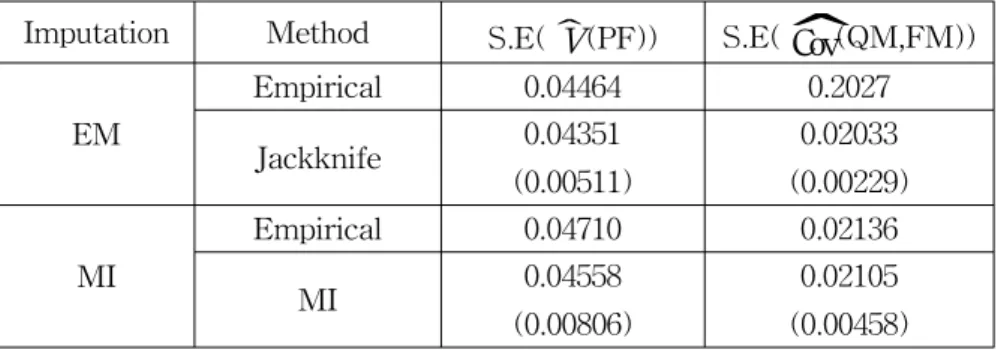
The table 1 shows the comparison of biases and efficiencies for the estimation of S.E(ˆV(PF)) and S.E(

ˆ

S.E(

ˆ

We can check biases through empirical values. When we compare the values between 'Empirical' and 'Jackknife' on 'EM' and 'MI', the jackknife estimation for EM algorithm and MI variance estimation are close to the empirical estimation.

It means that the variance estimates from the jackknife method for EM algorithm are unbiased and MI variance estimate is unbiased, too.

We can check the efficiency through the standard errors in the parenthesis. The jackknife method on EM algorithm provides more efficient variance estimation than MI variance estimation method.

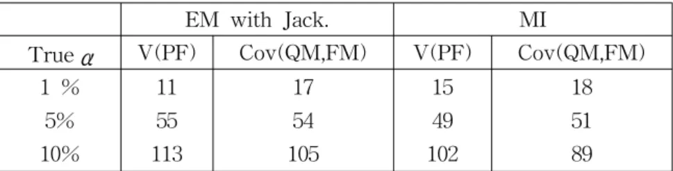
4.2 Comparison of Type I error levels

Let's consider tests for H₀:Var(PF)=0.49 and H₀:Cov(QM, FM)= 0.125 under α

= 0.01, 0.05 and 0.1. We can get the point estimation of Var(PF) and Cov(QM, FM) through the sample variance-covariance matrix from the EM algorithm, or MI procedure. Their standard errors are obtained from the EM algorithm. MI variance estimation procedure provides the standard error of the point estimation.

Then we can test it with assuming the jackknife distribution is approximately normal for 'EM'. Since S-Plus (2001) functions for MI give point estimation, standard errors and adjusted df, we can do t-test.

We have 1000 simulated data set and can test each data set. Table 2 shows the numbers of data sets for which the null hypothesis was falsely rejected out of 1000 data sets for three nominal Type I error levels. The EM with jackknife method and MI seem to have appropriate Type I error levels on both tests.

Table 1: Comparison of biases and efficiencies

Imputation Method S.E(ˆV_{(PF)) S.E(}

ˆ

Empirical 0.04464 0.2027

Jackknife 0.04351

(0.00511)

0.02033 (0.00229)

MI

Empirical 0.04710 0.02136

MI 0.04558

(0.00806)

0.02105 (0.00458)

Table 2: Comparison of Type I error levels

EM with Jack. MI

Trueα ^{V(PF) Cov(QM,FM) V(PF) Cov(QM,FM)}

1 % 5%

10%

11 55 113

17 54 105

15 49 102

18 51 89

5. Conclusion

The jackknife method on EM algorithm provides more efficient variance estimation than MI variance estimation method but the jackknife method on EM algorithm requires lots of computation. Multiple imputation requires less computation than resampling methods. However, the MI variance estimator tends to be larger than the Jackknife variance estimator with EM algorithm.

References

1. Dempster, A. P., Laird, N. M. and Rubin, D. B. (1977). Maximum likelihood from incomplete data via the EM algorithm(with discussion).

Journal of the Royal Statistical Society Series B, 39, 1-38.

2. Little, R. J. A. and Rubin, D. B. (2002). Statistical Analysis With Missing Data. J. Wiley & Sons, New York.

3. Rubin, D. B. (1976). Inference and missing data(with discussion).

Biometrika, 63, 581-592.

4. Rubin, D. B. (1978). Multiple imputation in sample surveys - A

phenomenological bayesian approach to nonresponse, Proceedings of the Survey Research Methods Section, American Statistical Association, 1978, 20-34

5. Kang, S. S. (2005). Comparison of EM and multiple imputation methods with traditional methods in monotone missing pattern. Journal of Korean Data & Information Science Society 2005, Vol. 16, No. 1, 95-106

6. S-Plus 6.1 Manual (2001). Analyzing Data With Missing Values in S-Plus, Insightful Corporation. Seattle, Washington.

[ received date : Sep. 2005, accepted date : Oct. 2005 ]