Similarity Measurement using Gabor Energy Feature and Mutual Information for Image Registration

1. Introduction

Image registration is one of the important steps to extract information from two or more images taken from the same scene at different times. Medical image analysis, object tracking in video images and image fusion are the application fields which need the image registration. Image registration is also an essential process to analyze the time series of satellite images in remote sensing fields such as change detection.

Image registration methods are often classified into two categories, pixel-based matching and feature- based matching techniques according to the image

feature (Zitova and Flusser, 2003). In feature-based matching techniques, highly informative features such as edges are used for matching(Han et al., 2011). In pixel-based matching techniques, on the other hand, image intensity values within a certain area are used for matching. The similarity measure which determines the corresponding pixels between two images is also important component. Mutual information (MI) is commonly used as similarity measure because of its robustness to noise (Cole- Rhodes, 2003; Suri and Reinartz, 2010). The MI- based registration methods employ the intensity information instead of image features. Due to the radiometric differences, it is not easy to apply MI to

Similarity Measurement using Gabor Energy Feature and Mutual Information for Image Registration

Chul-Soo Ye^†

Dept. of Ubiquitous IT, Far East University

Abstract :Image registration is an essential process to analyze the time series of satellite images for the purpose of image fusion and change detection. The Mutual Information (MI) is commonly used as similarity measure for image registration because of its robustness to noise. Due to the radiometric differences, it is not easy to apply MI to multi-temporal satellite images using directly the pixel intensity. Image features for MI are more abundantly obtained by employing a Gabor filter which varies adaptively with the filter characteristics such as filter size, frequency and orientation for each pixel. In this paper we employed Bidirectional Gabor Filter Energy (BGFE) defined by Gabor filter features and applied the BGFE to similarity measure calculation as an image feature for MI. The experiment results show that the proposed method is more robust than the conventional MI method combined with intensity or gradient magnitude.

Key Words :

Received October 29, 2011; Revised November 15, 2011; Accepted November 17, 2011.

†Corresponding Author: Chul-Soo Ye (csye@kdu.ac.kr)

multi-temporal satellite images using directly the pixel intensity. Butz and Thiran (2001) used edge measures instead of pixel intensity in similarity measure calculation. Lines and gradient information were also used in similarity measure calculation (Lehurea et al., 2008; Wen and Gau, 2009).

Image features are more abundantly obtained by employing the Gabor filter which varies adaptively with the filter characteristics such as filter size, frequency and orientation for each pixel. Gabor filter has been successfully employed in many image processing fields including image texture analysis (Dunn et al. 1994). In this paper we employ a local energy defined by Gabor filter features and apply the local energy to similarity measure calculation as an image feature for each pixel.

This paper is organized as follows: Gabor filter energy used as image feature and similarity measure calculation based on mutual information are described in Section 2. Image data used, results obtained and their analysis are given in Section 3.

Some conclusions are given in Section 4.

2. Methodology

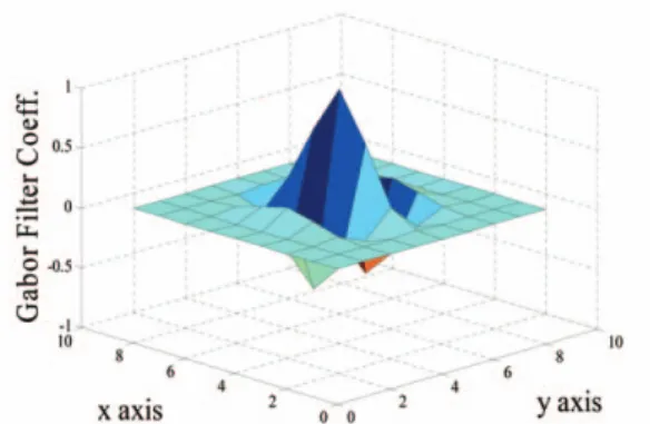
1) Bidirectional Gabor Filter Energy (BGFE) A Gabor filter is a linear filter obtained by product of a Gaussian kernel function and a complex sinusoidal signal. The two dimensional Gabor filters are given by the following form :

G

(x, y) = exp (_ ) ·exp{ j(2pfx

+ f)} (1) where

[ ] ⁼ [ ][ ]

and q

is the orientation of Gabor filter, f is the phase offset, s is the standard deviation of Gaussian

envelop and f is the frequency of the sinusoidal function. By adjusting q

, f and f, respectively, we can generate various types of Gabor filers. Fig. 1 shows Gabor filter coefficients in two dimensional space when q

=

/2, s = 1, f = 1/0.285 and f = 0.

Gabor Filter Energy (GFE) is defined as the square root of the sum of the squared response of even and odd symmetric filters, which is obtained by convolving the real and imaginary part, respectively, of the complex Gabor filter with an image as follows :

G

(x, y) = G

(x, y)

+ G

(x, y)

(2) where

G

(x, y) = I(x, y)ƒexp( ) ·cos(2pfx

+ f)

G

(x, y) = I(x, y)ƒexp( )·sin(2pfx

+ f) If we expand the equation (2) for more than one filter orientation, we find

G

(x, y) = G

(x, y)

+ G

(x, y)

,

(3) q

= (k _ 1), k = 1, 2, .., N

where N is the number of Gabor filter orientations.

For two filter orientations, p and q, we can define a Bidirectional Gabor Filter Energy (BGFE) as follows:

G

(x, y) = {G

(x, y)}

+ {G

(x, y)}

(4) p

N

x

+ y

2s

x

+ y

2s

x y cos

sin

sin

_ cos

x

y

x

+ y

2s

Korean Journal of Remote Sensing, Vol.27, No.6, 2011

Fig. 1. Example of Gabor filter coefficients (q_k = p/2, s = 1, f = 1/0.39 and f = 0).

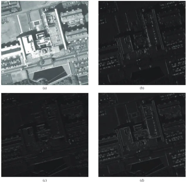
Though BGFE is similar to gradient magnitude in that it uses two filter orientations, BGFE is more flexible, however, in filter shape and orientation. The gradient magnitude is generally defined by the square root of the sum of the squared magnitude of vertical and horizontal gradients. BEFE, on the other hand, can be defined on various filter orientation and filter shape. For example, for N = 6, p = 2 and q = 5, we can compute the BGFE using Gabor filters rotated by

the two angles p/6 and 4p/6. In Fig. 2 (b) and (c) show GFE images when k = 1 and 4, respectively (N

= 6, f = 1/0.285, s = 1). The orientation difference of the two Gabor filters is p/2 . The BGFE image for p = 1 and q = 4 is shown in Fig. 2 (d). The BGFE image is used as image features in the calculation of the similarity measure.

Fig. 2. GFE and BGFE images (a) original image (b) GFE image (N = 6, k = 1, f = 1/0.285, s = 1) (c) GFE image (N = 6, k = 4, f = 1/0.285, s =1 ) (d) BGFE image (N = 6, p = 1, q = 4, f = 1/0.285, s = 1).

(c)

(a) (b)

(d)

2) Calculation of similarity measure based on mutual information

The Mutual Information (MI) is a basic concept in information theory. As a measurement of statistical correlation of two random variables, MI is used to calculate the similarity between two images. When the similarity between two images achieves a maximum, the MI of corresponding pixels used for similarity calculation also reaches a maximum value.

Denoting the features of the image A and B by the random variables, I

and I

, respectively, the MI is defined as follows:

MI(I

, I

) = H(I

) + H(I

) _ H(I

, I

) (5) where

H(I

) = _ p

(m)log p

(m) H(I

) = _ p

(n)log p

(n) H(I

, I

) = _ p

(m, n)log p

(m, n) where

p

(m), p

(n): marginal probability mass function p

(m, n): joint probability mass function

and the marginal probability mass function and joint probability mass function can be estimated from the feature (i.e., intensity, gradient magnitude, or BGFE) histogram of image A and B as follows :

p

(m) = , p

(n) = ,

p

(m, n) =

where m and n are the elements of the features of the image A and B, respectively.

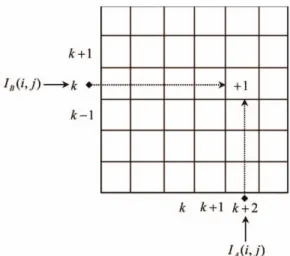
The cell of joint histogram counts the times at which the row and column of the 2-d histogram matrix have the feature element m of image A and the feature element n of the image B at a given image position (i, j), respectively. For example, when the

feature elements m and n are k and k + 2, respectively, at a given (i, j) position in image A and B as shown in Fig. 3., the number of bin at position (k, k + 2), h(k, k + 2), becomes h(k, k + 2)+1. This procedure is applied to all the pixels in the overlapping area of the two images.

As the feature of the image, intensity or gradient magnitude of the pixel is commonly used in calculation of similarity measure based on MI. In this paper, however, we used BGFE as the feature for similarity measure and compared the results with those of intensity-based MI and gradient-based MI.

3. Experimental Results

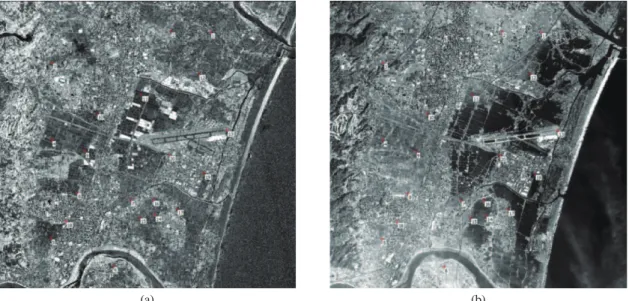
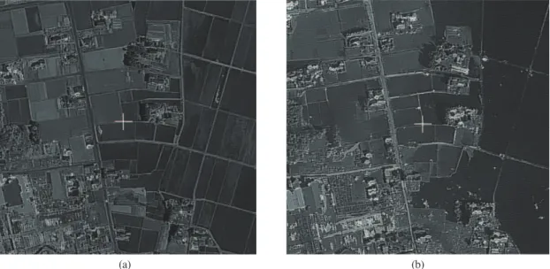
The proposed algorithm was tested using Kompsat-2 satellite images (Fig. 4). The Test images were taken over the tsunami affected areas of Sendai, Japan, on June 17, 2008 and on March 14, 2011, respectively. In Fig. 4(b), the dark areas within land are flooded areas by the tsunami. We chose 10 control points of non-flooded area and another 10 control points of flooded area in the matching window, respectively. The flooded areas in Fig. 4(b) h(m, n)

h(m, n) h(n)

h(n) h(m)

h(m)

S

S

S

S

Korean Journal of Remote Sensing, Vol.27, No.6, 2011

S

S

n m, n

S

Fig. 3. Example of joint histogram h(m, n) computation.

show more radiometric and geometric image change than the non-flooded areas after the tsunami.

For the images in Fig. 4, we generated BGFE images under the condition of p = 1, q = 4, N = 6, f = 1/0.285, s = 1. The BGFE images were used as image features for calculation of similarity measure based on MI. The size of the MI matching window for similarity measure is 601×601.

We found matches of the 20 control points in the left BGFE image (Fig. 5(a)) within the right BGFE image (Fig. 5(b)). Fig. 6 shows the 17th control point located at the center of the BGFE image of size 601

×601 in the flooded area. All the pixels in the matching window of size 601×601 are used in computation of the similarity measure. We look for the center positions of the matching window in both

(a) (b)

Fig. 5. BGFE images (a) June 17, 2008 (b) March 14, 2011.

(a) (b)

images at which the MI has maximum value. The two images show very different radiometric and geometric characteristics due to the damage of the tsumani. As image features, we also used intensity and gradient magnitude, respectively, to compare the matching results using intensity and gradient magnitude with BGFE matching results. Fig. 7 shows the matching results of the 20 control points for the three matching methods. For BGFE+MI method, the distribution of the errors of 10 control points (#1~#10) belonging to non-flooded areas and other

10 control points (#11~#20) belonging to flooded areas is more concentrated in the origin than other two methods.

Table 1, Talbe 2 and Table3 show the matching errors for each method. The mean row error for BGFE+MI method is 0.559, while the mean row errors for intensity+MI and gradient magnitude+MI methods are 0.659 and 0.623, respectively. The mean column error for BGFE+MI method is 0.679, while the mean column errors for intensity+MI and gradient magnitude+MI methods are 0.847 and 0.708,

Korean Journal of Remote Sensing, Vol.27, No.6, 2011

Fig. 6. The 17^thcontrol point at the center of the BGFE images (a) June 17, 2008 (b) March 14, 2011.

(a) (b)

Fig. 7. Matching errors of the 20 control points. The small circles represent the errors of the 10 control points belonging to non- flooded areas and the small diamonds represent the errors of 10 control points of flooded areas (a) intensity feature + MI (b) gradient magnitude + MI (c) BGFE + MI.

(a) (b) (c)

respectively. The BGFE+MI method also showed better performance for the control points in both non- flooded and flooded areas than other two methods.

We applied the proposed algorithm to another pair of Kompsat-2 images (Fig. 8). We added another Kompsat-2 image taken on March 29, 2011 as shown in Fig. 8(b). Table 4, Table 5 and Table 6 show the

matching errors for the intensity+MI method, gradient magnitude+MI method and the BGFE+MI method, respectively. The BGFE+MI method shows better matching performance than other two methods.

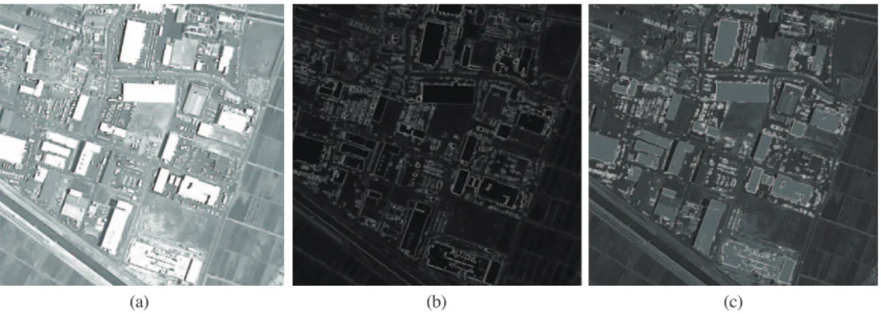
Fig. 9 shows the characteristics of the BGFE image compared to intensity image and gradient magnitude image. In the BGFE image, both the high gradient

Control Points(CP) Row error (mean) Column error (mean)

10 CPs (# 1 ~ #10) 0.584 0.886

10 CPs (#11 ~ #20) 0.847 1.227

20 CPs (Total) 0.715 1.057

Control Points(CP) Row error (mean) Column error (mean) Table 1. Matching errors for the intensity+MI method

Control Points(CP) Row error (mean) Column error (mean)

10 CPs (# 1 ~ #10) 0.517 0.706

10 CPs (#11 ~ #20) 0.800 0.989

20 CPs (Total) 0.659 0.847

Control Points(CP) Row error (mean) Column error (mean)

Table 2. Matching errors for the gradient magnitude+MI method

Control Points(CP) Row error (mean) Column error (mean)

10 CPs (# 1 ~ #10) 0.645 0.606

10 CPs (#11 ~ #20) 0.601 0.810

20 CPs (Total) 0.623 0.708

Control Points(CP) Row error (mean) Column error (mean)

Table 3. Matching errors for the BGFE+MI method

Control Points(CP) Row error (mean) Column error (mean)

10 CPs (# 1 ~ #10) 0.517 0.606

10 CPs (#11 ~ #20) 0.601 0.789

20 CPs (Total) 0.559 0.697

Control Points(CP) Row error (mean) Column error (mean)

Table 6. Matching errors for the BGFE+MI method

Control Points(CP) Row error (mean) Column error (mean)

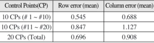
10 CPs (# 1 ~ #10) 0.545 0.688

10 CPs (#11 ~ #20) 0.847 1.127

20 CPs (Total) 0.696 0.908

Control Points(CP) Row error (mean) Column error (mean)

Fig. 8. Kompsat-2 satellite images over Sendai, Japan taken (a) on June 17, 2008 (b) on March 29, 2011.

(a) (b)

Table 4. Matching errors for the intensity+MI method

Control Points(CP) Row error (mean) Column error (mean)

10 CPs (# 1 ~ #10) 0.784 0.991

10 CPs (#11 ~ #20) 0.947 1.127

20 CPs (Total) 0.865 1.127

Control Points(CP) Row error (mean) Column error (mean)

magnitudes of pixels (bright pixels in Fig. 9(c)) and texture information of non-edge areas were well preserved. Due to these two characteristics of high gradient magnitude and texture information preservation in the BGFE image, the BGFE+MI method showed better performance in the matching results.

4. Conclusions

The image registration is an essential process to analyze the time series of satellite images. For the images containing the effect of natural disasters such as floods, it is difficult to find correct matched points due to the radiometric and geometric changes before and after the natural disaster. This paper proposed a new method for similarity calculation by using the Bidirectional Gabor Filter Energy (BGFE) and mutual information for the registration between the images containing some radiometric and geometric changes. The proposed BGFE+MI method showed better matching performance compared to the intensity+MI method and the gradient magnitude+MI method. The future direction is that the shape of the matching window can be further extended to fit the registration between rotated images.

Acknowledgements

This research was supported by a grant by Satellite Information Application Supporting Program of Satellite Information Research Center in Korea Aerospace Research Institute in 2011.

References

Butz, T. and J.P. Thiran, 2001. Affine registration with feature space mutual information, Proc.

MICCAI, Lecture Notes in Computer Science, W. Niessen and M. Viergerver, Eds., Berlin, Germany, 2208:549-556.

Cole-Rhodes, A.A., K.L. Johnson, J. LeMoigne, and I. Zavorin, 2003. Multiresolution registration of remote sensing imagery by optimization of mutual information using a stochastic gradient, IEEE Transactions on Image Processing, 12(12):1495-1511.

Dunn, D., W.E. Higgins, and J. Wakeley, 1994.

Texture segmentation using 2D Gabor elementary functions, IEEE Transactions on Pattern Analysis and Machine Intelligence, 16(2): 130-149.

Han, Y.K., D.J. Kim, and Y.I. Kim, 2011.

Korean Journal of Remote Sensing, Vol.27, No.6, 2011

Fig. 9. Sample images (a) intensity image (b) gradient magnitude image (c) BGFE image.

(a) (b) (c)

Registration between High-resolution Optical and SAR Images Using Linear Features, Korean Journal of Remote Sensing, 17(2):

141-150.

Lehureau, G., F. Tupin, C. Tison, G. Oller, and D.

Petit, 2008. Registration of metric resolution SAR and optical images in urban areas, European conference on synthetic aperture radar; EUSAR 2008, 197-200.

Suri, S. and P. Reinartz, 2010. Mutual-information- based registration of TerraSAR-X and Ikonos

Imagery in urban areas, IEEE Transactions on Geoscience and Remote Sensing, 48(2):

939-949.

Wen, H.Y. and J.T. Gao, 2009. Remote sensing image registration based on mutual information and grey relational analysis, IEEE International Conference on Intelligent Computing and Intelligent Systems, 4: 127- 131.

Zitova, B. and J. Flusser, 2003. Image registration

methods: a survey, Image and Vision Computing,

21: 977-1000.