Two-Stage Logistic Regression for Cancer Classification and Prediction from Copy-Number Changes in cDNA Microarray-Based Comparative
Genomic Hybridization
Mijung Kim1
1Institute for Mathematical Sciences, Yonsei University (Received June 2011; accepted August 2011)
Abstract
cDNA microarray-based comparative genomic hybridization(CGH) data includes low-intensity spots and thus a statistical strategy is needed to detect subtle differences between different cancer classes. In this study, genes displaying a high frequency of alteration in one of the different classes were selected among the pre-selected genes that show relatively large variations between genes compared to total variations.
Utilizing copy-number changes of the selected genes, this study suggests a statistical approach to predict patients’ classes with increased performance by pre-classifying patients with similar genetic alteration scores.
Two-stage logistic regression model(TLRM) was suggested to pre-classify homogeneous patients and predict patients’ classes for cancer prediction; a decision tree(DT) was combined with logistic regression on the set of informative genes. TLRM was constructed in cDNA microarray-based CGH data from the Cancer Metas- tasis Research Center(CMRC) at Yonsei University; it predicted the patients’ clinical diagnoses with perfect matches (except for one patient) among the high-risk and low-risk classified patients where the performance of predictions is critical due to the high sensitivity and specificity requirements for clinical treatments. Ac- curacy validated by leave-one-out cross-validation(LOOCV) was 83.3% while other classification methods of CART and DT performed as comparisons showed worse performances than TLRM.
Keywords: cDNA microarray-based comparative genomic hybridization, gene copy-number change, pre- dicted probability, decision tree, factor analysis, logistic regression model.
1. Introduction
Many defects in human development are known to be due to gains and losses of chromosomes and chromosomal segments. Changes in DNA copy-number in somatic cells have been shown to contribute to the development of cancer (Pinkel and Albertson, 2005). Therefore, a better This work was supported by Basic Science Research Program through the National Research Founda- tion(NRF) funded by the Ministry of Education, Science and Technology(MEST) (NRF-2008-532-C00046).
1Research Professor, Institute for Mathematical Sciences, Yonsei University, 134 Shinchon-Dong, Seodaemun-Gu, Seoul 120-752, Korea. E-mail: mjkim@yonsei.ac.kr
understanding of the effects of changes in DNA copy number may help identify and validate potential cancer genes (Mestre-Escorihuela et al., 2007). Comparative genomic hybridization(CGH) using cDNA microarrays can identify disease-related DNA copy number changes and make it possible to observe diverse patterns of potential biomarkers and/or related genes at the DNA level. cDNA microarray-based CGH is a useful technique to detect genome aberrations with high resolution; a genomic alteration detected by cDNA microarray-based CGH can be easily translated into sequence and gene identification to provide additional information in regards to chromosomal rearrangements and imbalances (Squire et al., 2003). Using cDNA clones instead of BAC or PAC clones as probes would make it possible to directly detect amplification and deletion of copy numbers of individual genes (Kawaguchi et al., 2005).
A gastric cancer related cDNA microarray-based CGH experiment was performed to delineate individual genes that undergo copy-number changes with a high resolution at the Cancer Metastasis Research Center(CMRC) at Yonsei University. For gene-by-gene identification of copy-number changes in CGH experiment, Yang S. H. et al., performed simple frequency analysis and selected genes that showed at least one alteration in gastric cancer with the same cDNA microarray-based CGH data mentioned above (Yang et al., 2005). Cheng et al. (2003) analyzed array CGH based on a gene-by-gene search through array rank order to detect copy-number changes in human cancer (Cheng et al., 2003).
Readers can refer to the article (Yang et al., 2005) that worked with the same data as this present study to select genes related to the recurrence of gastric cancer. To score genetic information, they related the summation of changes in the number of gene copies of amplified genes (without considering deletions) to the recurrence of cancer.
As means of scoring genetic information, Inoue et al., assigned a weight of +1 or −1 to the gene depending on its characteristic for the five conventional pathological factors in relation to gastric cancer (Inoue et al., 2002); Liu et al., suggested a linear transformation method for cancer classifi- cation using rotation forest (Liu and Huang, 2008); A study by Kim and Chung considered the gain as well as the loss in the number of gene copies and a weight was assigned to each gene according to its contribution to the genetic score related to the risk of recurrence (Kim and Chung, 2009).
In this present study for the cDNA microarray-based CGH data of CMRC, genes altered in gastric cancer and that could be used to distinguish different classes (cancer stages) were first collected.
To assign a weight to each gene to score genetic information, a few linear combinations of those collected genes were sought so that they were orthogonal and were independent components. Each linear combinations of these collected, informative genes was named genetic alteration score(GAS) which is the weighted sum of informative genes. A logistic regression approach that employs a decision tree(DT) was developed to pre-classify homogeneous patients and predicting cancer stage of patients, and predict the cancer stage of patients; we named it the two-stage logistic regression model(TLRM). The gene’s impact on risk factors were possibly examined with the correlations of GASs for each gene.
This study was done with the following process: (a) to determine the set of informative genes(SIG) that displayed a high frequency of alteration on one of the two cancer stages and to select significant genes in SIG; (b) to relate copy-number changes of the significant genes in SIG with the patient’s cancer stage; (c) to create a patient’s index to pre-classify homogeneous patients and to develop a predictive model for patients’ classes for cancer prediction.
‘Materials and methods’ section described data preparation, SIG, and how to construct TLRM with
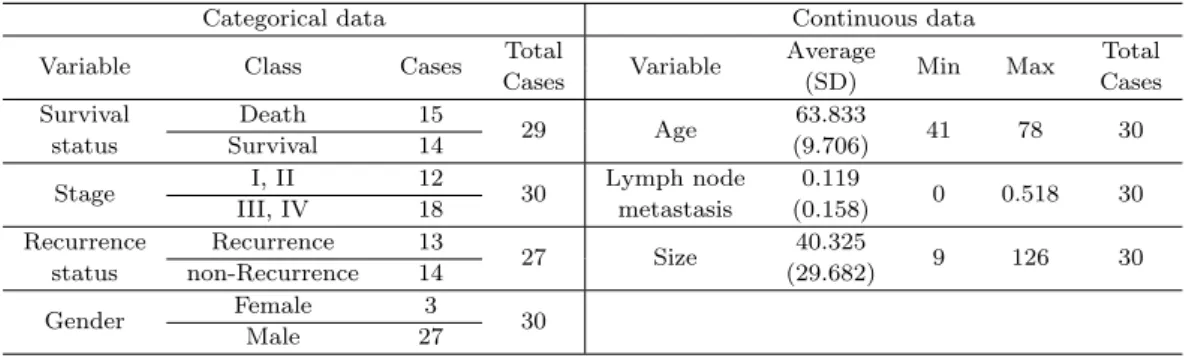
Table 2.1. Clinical information of thirty patients for the 65 months follow-up study
Categorical data Continuous data
Variable Class Cases Total
Variable Average
Min Max Total
Cases (SD) Cases
Survival Death 15
29 Age 63.833
41 78 30
status Survival 14 (9.706)
Stage I, II 12
30 Lymph node 0.119
0 0.518 30
III, IV 18 metastasis (0.158)
Recurrence Recurrence 13
27 Size 40.325
9 126 30
status non-Recurrence 14 (29.682)
Gender Female 3
Male 27 30
the establishment of GAS. ‘Results’ section showed TLRM constructed with the data of CMRC from Yonsei University and explanation on characteristics of GAS. The probability for a patient’s late- cancer stage, named predicted score(PS) and its application were also described. The status of the cancer stage was predicted using PS. In addition, a comparison with other classification methods was discussed.
2. Materials and Methods
Gastric cancer related cDNA microarray-based CGH data were obtained from the CMRC at Yonsei University. Briefly, thirty pairs of normal gastric mucosa and cancer tissues were obtained from gas- tric cancer patients at Severance Hospital, Yonsei University Health System, Seoul, Korea, from 1997 to 1999. The cDNA microarrays containing 17K human gene probes (CMRC-Genomictree, Korea) were used for CGH following the standard protocol of CMRC, Yonsei University (Yang et al., 2005;
Park et al., 2006). In this experiment, normal and tumor genomic DNA samples were extracted from the same patient and hybridized on the same spotted array. 17K cDNA microarray contained the 15,723 unique genes with 17,664 spots and these unique genes were mapped for their chromoso- mal location using SOURCE (http://genome-www5.stanford.edu/cgi-bin/source/sourceSearch) and DAVID (http://apps1.niaid.nih.gov/david/). Clinical data description is shown in Table 2.1.
2.1. Data preparation
The transformation of the intensity signal to a ratio was carried out using the log2red to green ratio, log2(R/G), where R and G denote the fluorescent intensities of tumor and normal hybridizations, respectively. Data was pre-processed with the following steps: within-print tip, intensity-dependent normalization of Y (Yang et al., 2002), deletion of genes showing missing values for > 20% of the total number of observations, employment of a 10-nearest neighbor method for the imputation of missing values, and averaging values for the case of the multiple spots. Following these steps 10,514 genes were found from the 30 microarrays. The set of this data was used as the initial set for analysis, and filtering genes with a reproducible gene selection algorithm(RGSA) (Kim, 2009) was performed on this set.
Park et al. evaluated genome-wide measurement of the copy-number of each gene in normal gastric cancer and placenta tissues to determine the criteria on a genomic alteration with the same data of cDNA microarray-based CGH; the range of genomic copy number of normal tissues was found
to be±0.3 of the log2 fluorescence intensity ratio in the autosomal genes (Park et al., 2006). This criterion was used to categorize the gene’s copy-number change into alteration and non-alteration.
The cDNA microarray-based CGH data for this study has been deposited into Array Express (http://www.ebi.ac.uk/arrayexpress/) Query:1283947172 E-TABM-171. Data analysis was per- formed with SAS V.9.1.
2.2. Set of informative genes(SIG)
We considered the set of genes that show a high frequency of alteration in one of the different cancer classes as informative genes of being different in copy-number changes between different cancer classes in cDNA microarray-based CGH; based on the selected genes in SIG, GASs were established with the purpose for scoring patients’ genetic information so that a patient’s PS was obtained for to assess the risk of the late-cancer stage. Since cDNA microarray based CGH data included low-intensity spots, a statistical strategy to detect subtle differences between different classes (two cancer stages) was needed. For this purpose, genes with relatively large variations between genes compared to total variations were first pre-selected. Of those pre-selected genes, genes displaying a high frequency of alteration in either early-cancer stage(ES; cancer stage I or II) or late-cancer stage(LS; cancer stage III or IV) were selected. We determined the set of selected genes as SIG with the criteria of an increased reproducibility and a reasonable number of genes utilized for the classifier.
In pattern recognition, we usually adopt the following criterion: the smaller is the sum of squares within genes and the bigger is the sum of squares between genes, the better is the classification accuracy. Therefore we define reproducibility using the above two statistics to pre-select genes; the reproducibility was measured with the ratio of intrinsic variation of genes which is the extent of the
‘between-gene’ variation, to the sum of the intrinsic variation of genes and the variation between arrays that include measurement error, which is the ‘within-gene’ variation. This ratio explains how closely the gene measurements of one array track the gene measurements of another; a large reproducibility makes it easy to measure a change in the copy-number for the gene (Kim, 2009).
Using reproducible gene selection algorithm(RGSA) we collect genes with relatively large variations between genes compared to total variation, which results in the increment of reproducibility for the set of remaining genes. At this stage, two types of pre-selected sets were considered; the initial set, INI that includes all genes without a consideration of variations after within-print tip, intensity- dependent normalization (INI had a reproducibility of 17.24% for the CMRC data of this study);
the filtered set, Sf ilt obtained by maximizing both reproducibility and the number of remaining genes (Sf ilt had a reproducibility of 24.5% for the CMRC data).
For the number of genes utilized for classifier, in the first place, genes in each set were categorized into the non-alteration/alteration group; the range of genomic copy number of normal tissues was found to be±0.3 of the log2fluorescence intensity ratio in the autosomal genes (Park et al., 2006) and this criterion was used to categorize the gene’s copy-number change into alteration and non-alteration.
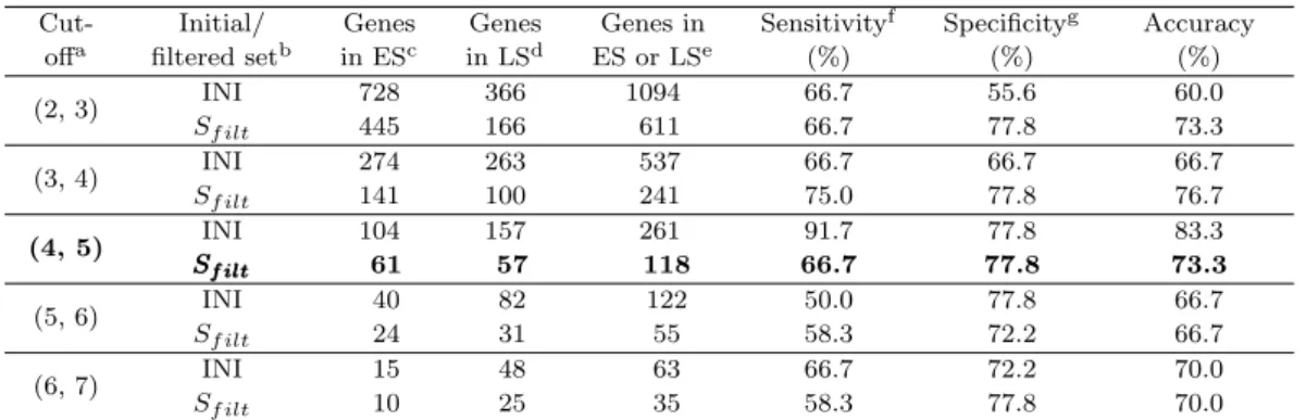
To utilize copy-number changes to separate cancer stages, genes with a frequency of alteration at least 20% in either early-cancer or late-cancer group are collected; consideration was made from the set of genes with frequency cut-off of 2 and 3 for the early- and the late-cancer stage group, respectively, up to the set consisted of about 50 genes; each case was denoted (2, 3), (3, 4), . . . , (6, 7) and the notation, for example, (2, 3) is the set of genes where genes have at least a frequency of alterations of 2 and 3 for early- and late-cancer stage group, respectively. Table 2.2 displays reproducibility for the corresponding cut-off and number of genes utilized for the classifier.
Table 2.2. Classification rates validated with cross-validation
Cut- Initial/ Genes Genes Genes in Sensitivityf Specificityg Accuracy
offa filtered setb in ESc in LSd ES or LSe (%) (%) (%)
(2, 3) INI 728 366 1094 66.7 55.6 60.0
Sf ilt 445 166 611 66.7 77.8 73.3
(3, 4) INI 274 263 537 66.7 66.7 66.7
Sf ilt 141 100 241 75.0 77.8 76.7
(4, 5) INI 104 157 261 91.7 77.8 83.3
Sf ilt
SSf iltf ilt 61 57 118 66.7 77.8 73.3
(5, 6) INI 40 82 122 50.0 77.8 66.7
Sf ilt 24 31 55 58.3 72.2 66.7
(6, 7) INI 15 48 63 66.7 72.2 70.0
Sf ilt 10 25 35 58.3 77.8 70.0
a: Frequency cut-off for finding ‘high’ frequency of alteration in early- and late-cancer stage, respectively;
b: Initial/ filtered set for increasing reproducibility; a reproducibility of 17.24% and 24.5% for INI and Sf ilt of the CMRC data, respectively; c, d: Number of genes showed a high frequency of alteration in early-cancer(ES) and late-cancer stage(LS), respectively; e: Total number of genes utilized for the classi- fier; f, g: Sensitivity and specificity were investigated on the event of occurrence for late-cancer stage.
The set boldfaced was selected as a SIG for this study. The accuracy of the classifications was tested by cross-validation; one withheld a sample, built a logistic regression model with GASs based on the genes collected only from the remaining samples, and predicted the class of the withheld sample. The process was repeated for each sample, and the cumulative error rate was calculated.
As a default, we recommend trying the set of 50 to 250 genes from the set with reproducibility increased, although this recommendation is somewhat arbitrary. As Table 2.2 shows, the set with cut-off (4, 5) or (5, 6) consisted of 55 to 261 genes at INI or Sf ilt where Sf ilt keeps increased reproducibility comparing to INI; we select the set Sf ilt with cut-off (4, 5) as SIG since it consisted of a reasonable number of genes that express a high frequency of alteration (about 30%) in one of the two stages.
2.3. Constructing two-stage logistic regression model(TLRM)
Of the 118 genes in SIG, 28 genes that show statistical significances in difference between the two different cancer stages were selected to construct a GAS that could score a patient’s risk of the late-cancer stage. At the first stage of TLRM, we utilized DT to pre-classify patients with similar GASs by relating copy-number changes of the 28 genes compiled from SIG with patient’s cancer stage. Once such subgroups were created, at the second stage of TLRM, we employed a supervised learning technique, logistic regression to predict future patients’ classes to improve its performance by incorporating a patient’s index and continuous predictor(s) of patients’ classes into the model;
it showed an improved performance of predictions for the patients classified into high- and low-risk on whom predictions should be critical as they require a high sensitivity on the high-risk patients (a high specificity on the low-risk patients) for decisions on clinical treatments.
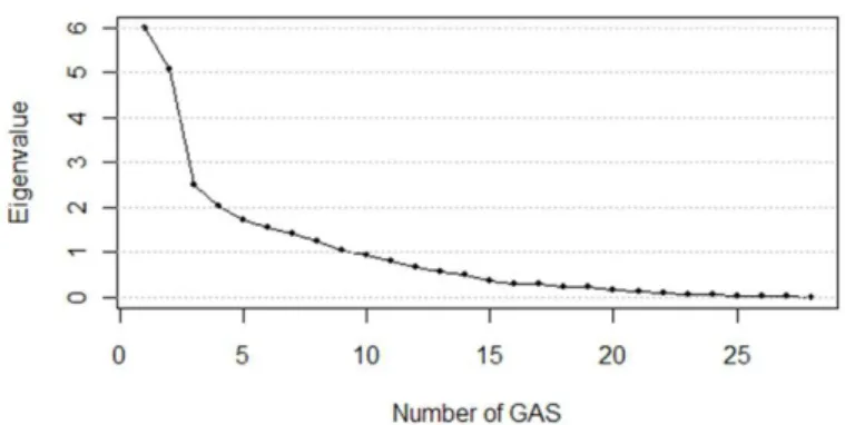
For the calculation of patients’ GASs, the characteristics of the 28 genes in SIG were decomposed into several common characteristics by performing factor analysis with principal component analy- sis(PCA). The number of factors was determined at a level that showed an eigenvalue greater than 1.0 and cumulative variability of at least 80%; the top nine factors (the factor scores were named GASs), were determined as shown in Figure 2.1. The orthogonal factor model was constructed with these nine GASs that are linear combinations of the selected 28 genes.
Figure 2.1. Scree plot for the proportions of variability explained by GASs(x- and y-axis represent factor number and eigen value for the proportion of variability explained by the corresponding factor.)
Each gene had correlations with the nine GASs (shown with rotated GAS patterns in Table 2.3) as GAS loadings, which are correlations between each gene and the corresponding GAS. GASs were derived so that they were orthogonal, and the genes’ weights were used to obtain GASs; each of the GASs was denoted GAS1, GAS2, . . . and so on.
Once patients’ GASs were obtained, DT was built to investigate homogeneous patients with regard to their GASs and deal with interactions between the nine GASs. For optimal tree selection, the number of leaves was determined where the overall misclassification rate committed on all folds in the leave-one-out cross-validation was greatly reduced and became steady thereafter; these tree subgroups were subject to χ2 statistic where the final split value was determined by χ2 statistic whose p-value is minimized among all possible splits, and each subgroup was determined by the final split value. The patient’s index variable was created based on the interacting GASs found from DT; by employing this index, patients can be assigned to a high-risk, an in-between risk or a low-risk subgroup according to their GASs; however, sometimes a continuous predictor of patients’
classes is desired. We employ GASs that can be used to calculate a continuous risk score for a given patient. The resulting predictor improves its performance when applied to logistic regression for cancer prediction. Thus, the patients’ GASs together with the patient’s index were employed into the logistic regression as explanatory variables. The nine GASs were examined with variable selection in an attempt to detect GASs that would affect the risk of late-cancer stage.
The suggested two-stage logistic regression with p explanatory variables and patient’s index I was then expressed as
ln
{Pr (Y = 1|X1, . . . , Xp) Pr (Y = 0|X1, . . . , Xp) }
= β0+ β1x1+· · · + βpxp+ γI,
where Y was a dependent variable representing whether a patient’s cancer was in the late-cancer stage or not, and a value of 1 was used for late-cancer stage and 0 otherwise. β0, . . . , βpand γ were regression coefficients. Patient’s index I was created to employ significant interactions between GASs and to pre-classify homogeneous patients.
3. Results
The result of DT analysis is shown in Figure 3.1; for determination of optimal tree, sensitivity
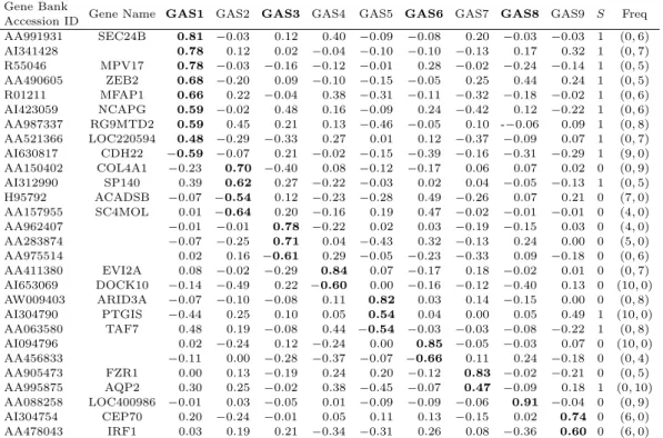
Table 2.3. Rotated GAS patterns for the 28 informative genes Gene Bank
Gene Name GAS1 GAS2 GAS3 GAS4 GAS5 GAS6 GAS7 GAS8 GAS9 S Freq
Accession ID
AA991931 SEC24B 0.81 −0.03 0.12 0.40 −0.09 −0.08 0.20 −0.03 −0.03 1 (0, 6)
AI341428 0.78 0.12 0.02 −0.04 −0.10 −0.10 −0.13 0.17 0.32 1 (0, 7)
R55046 MPV17 0.78 −0.03 −0.16 −0.12 −0.01 0.28 −0.02 −0.24 −0.14 1 (0, 5) AA490605 ZEB2 0.68 −0.20 0.09 −0.10 −0.15 −0.05 0.25 0.44 0.24 1 (0, 5) R01211 MFAP1 0.66 0.22 −0.04 0.38 −0.31 −0.11 −0.32 −0.18 −0.02 1 (0, 6) AI423059 NCAPG 0.59 −0.02 0.48 0.16 −0.09 0.24 −0.42 0.12 −0.22 1 (0, 6) AA987337 RG9MTD2 0.59 0.45 0.21 0.13 −0.46 −0.05 0.10 -−0.06 0.09 1 (0, 8) AA521366 LOC220594 0.48 −0.29 −0.33 0.27 0.01 0.12 −0.37 −0.09 0.07 1 (0, 7) AI630817 CDH22 −0.59 −0.07 0.21 −0.02 −0.15 −0.39 −0.16 −0.31 −0.29 1 (9, 0) AA150402 COL4A1 −0.23 0.70 −0.40 0.08 −0.12 −0.17 0.06 0.07 0.02 0 (0, 9) AI312990 SP140 0.39 0.62 0.27 −0.22 −0.03 0.02 0.04 −0.05 −0.13 1 (0, 5) H95792 ACADSB −0.07 −0.54 0.12 −0.23 −0.28 0.49 −0.26 0.07 0.21 0 (7, 0) AA157955 SC4MOL 0.01 −0.64 0.20 −0.16 0.19 0.47 −0.02 −0.01 −0.01 0 (4, 0)
AA962407 −0.01 −0.01 0.78 −0.22 0.02 0.03 −0.19 −0.15 0.03 0 (4, 0)
AA283874 −0.07 −0.25 0.71 0.04 −0.43 0.32 −0.13 0.24 0.00 0 (5, 0)
AA975514 0.02 0.16 −0.61 0.29 −0.05 −0.23 −0.33 0.09 −0.18 0 (0, 6)
AA411380 EVI2A 0.08 −0.02 −0.29 0.84 0.07 −0.17 0.18 −0.02 0.01 0 (0, 7) AI653069 DOCK10 −0.14 −0.49 0.22 −0.60 0.00 −0.16 −0.12 −0.40 0.13 0 (10, 0) AW009403 ARID3A −0.07 −0.10 −0.08 0.11 0.82 0.03 0.14 −0.15 0.00 0 (0, 8)
AI304790 PTGIS −0.44 0.25 0.10 0.05 0.54 0.04 0.00 0.05 0.49 1 (10, 0)
AA063580 TAF7 0.48 0.19 −0.08 0.44 −0.54 −0.03 −0.03 −0.08 −0.22 1 (0, 8)
AI094796 0.02 −0.24 0.12 −0.24 0.00 0.85 −0.05 −0.03 0.07 0 (10, 0)
AA456833 −0.11 0.00 −0.28 −0.37 −0.07 −0.66 0.11 0.24 −0.18 0 (0, 4)
AA905473 FZR1 0.00 0.13 −0.19 0.24 0.20 −0.12 0.83 −0.02 −0.21 0 (0, 5) AA995875 AQP2 0.30 0.25 −0.02 0.38 −0.45 −0.07 0.47 −0.09 0.18 1 (0, 10) AA088258 LOC400986 −0.01 0.03 −0.05 0.01 −0.09 −0.09 −0.06 0.91 −0.04 0 (0, 9) AI304754 CEP70 0.20 −0.24 −0.01 0.05 0.11 0.13 −0.15 0.02 0.74 0 (6, 0)
AA478043 IRF1 0.03 0.19 0.21 −0.34 −0.31 0.26 0.08 −0.36 0.60 0 (6, 0)
The GAS patterns of the nine GASs were shown. Entries are GAS loadings that are correlations of each gene with the corresponding GASs. GAS loadings boldfaced are strong correlations of the genes with the correspon- ding GAS and those corresponding genes represent the characteristic of the corresponding GAS when compared to the other GASs.
S: Gene’s status on alteration of high frequency (0 = high frequency in early-cancer stage; 1 = high frequency in late-cancer stage).
Freq: Frequency of gains & losses over the thirty patients, (m, n) for m gains and n losses, respectively. For ins- tance, Gene Bank Accession ID AA991931 showed alteration of high frequency in patients of late-cancer stage (S = 1), 6 losses but no gains, and non-alterations of the remaining twenty-four patients from among the thirty patients.
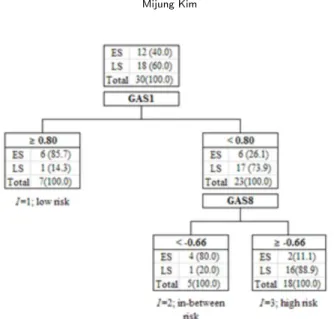
analysis was performed using cross-validation technique before utilizing the full data set. (One withheld a sample to test DT which was built with the rest of the samples. This step was repeated for each sample. At the number of leaves three, the overall misclassification rate committed on all folds was greatly reduced and became steady thereafter.) The final DT was built based on the full data set. Their best splits were 0.80 and−0.66 for GAS1 and GAS8, respectively, and these splits were determined based on χ2statistic whose p-values were minimized among all possible splits. The most homogeneous tree subgroups subject to χ2 statistic were determined with these split values.
The index I was employed to sign homogeneous patients to low-risk, in-between risk, or high-risk for patients with ‘GAS1≥ 0.80’, ‘GAS1 < 0.80 & GAS8 < −0.66’, or ‘GAS1 < 0.80 & GAS8 ≤ −0.66’, respectively. This index assigns each patient a score based on the patient’s risk for late-cancer; 1, 2, and 3 for low risk, in-between risk, and high risk, respectively (Equation (3.1) & Figure 3.1).
Using a stepwise variable selection, the index I, GAS3, and GAS6 were shown to be significant risk factors; the selection levels for entering and removing a variable were 0.1 and 0.15, respectively (Table 3.1).
Figure 3.1. Result of DT analysis (The optimal split-values for the GAS1 and GAS8 are 0.80 and−0.66, respectively. The number of patients is written in the corresponding leaf, and % is in parenthesis. ES: early-cancer stage, LS: late-cancer stage)
Table 3.1. Results of analysis using the suggested model, TLRM (Selected factors with TLRM)
Parameter DF Estimate Standard Error Wald Chi-Sq Pr > Chi-Sq Estimate of odds ratio
Intercept 1 −8.29 3.16 6.91 0.09
GAS3 1 −1.70 0.95 3.18 0.07 0.18
GAS6 1 −2.01 1.13 3.14 0.08 0.13
I 1 3.98 1.52 6.83 0.01 53.28
Based on the results shown in Table 3.1, the fitted model for a patient’s cancer stage was constructed as follows:
ln
{ Pr(late cancer stage| GAS1, GAS3, GAS6, GAS8) Pr(early cancer stage| GAS1, GAS3, GAS6, GAS8)
}
=−8.29 − 1.70GAS3 − 2.01GAS6 + 3.98I, (3.1)
where I =
{1, if GAS1≥ 0.80,
2, if GAS1 < 0.80 & GAS8 <−0.66, 3, if GAS1 < 0.80 & GAS8≥ −0.66.
GAS1 and GAS8 were interacting factors in relation to the risk of late-cancer stage, and GAS3 and GAS6 were additionally selected as risk factors in the suggesting TLRM; GAS1 which shows the largest eigenvalue among the nine GASs had the first priority as a criterion for grouping homoge- neous patients. For each gastric cancer patient, the predicted probability, called PS, was obtained by
Pr(late cancer stage| GAS1, GAS3, GAS6, GAS8)
= exp(−8.29 − 1.70GAS3 − 2.01GAS6 + 3.98I)
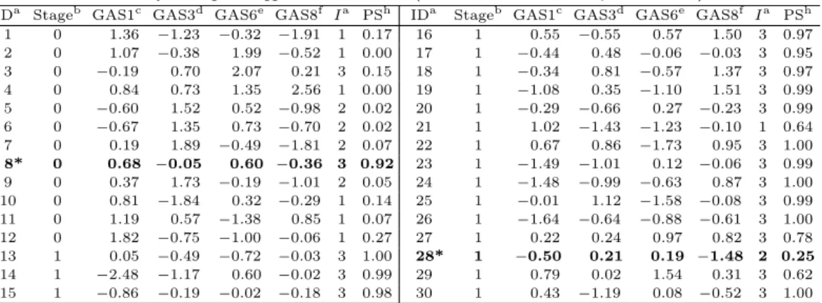
1 + exp(−8.29 − 1.70GAS3 − 2.01GAS6 + 3.98I). (3.2) In Table 3.2, the thirty patients’ GASs, indices of being assigned, and PSs obtained by the predicted score are listed.
Table 3.2. Results of analysis using the suggested model, TLRM (Patient’s GASs, index, and predicted score)
IDa Stageb GAS1c GAS3d GAS6e GAS8f Ia PSh IDa Stageb GAS1c GAS3d GAS6e GAS8f Ia PSh 1 0 1.36 −1.23 −0.32 −1.91 1 0.17 16 1 0.55 −0.55 0.57 1.50 3 0.97 2 0 1.07 −0.38 1.99 −0.52 1 0.00 17 1 −0.44 0.48 −0.06 −0.03 3 0.95 3 0 −0.19 0.70 2.07 0.21 3 0.15 18 1 −0.34 0.81 −0.57 1.37 3 0.97 4 0 0.84 0.73 1.35 2.56 1 0.00 19 1 −1.08 0.35 −1.10 1.51 3 0.99 5 0 −0.60 1.52 0.52 −0.98 2 0.02 20 1 −0.29 −0.66 0.27 −0.23 3 0.99 6 0 −0.67 1.35 0.73 −0.70 2 0.02 21 1 1.02 −1.43 −1.23 −0.10 1 0.64 7 0 0.19 1.89 −0.49 −1.81 2 0.07 22 1 0.67 0.86 −1.73 0.95 3 1.00 8* 0 0.68 −0.05 0.60 −0.36 3 0.92 23 1 −1.49 −1.01 0.12 −0.06 3 0.99 9 0 0.37 1.73 −0.19 −1.01 2 0.05 24 1 −1.48 −0.99 −0.63 0.87 3 1.00 10 0 0.81 −1.84 0.32 −0.29 1 0.14 25 1 −0.01 1.12 −1.58 −0.08 3 0.99 11 0 1.19 0.57 −1.38 0.85 1 0.07 26 1 −1.64 −0.64 −0.88 −0.61 3 1.00 12 0 1.82 −0.75 −1.00 −0.06 1 0.27 27 1 0.22 0.24 0.97 0.82 3 0.78 13 1 0.05 −0.49 −0.72 −0.03 3 1.00 28* 1 −0.50 0.21 0.19 −1.48 2 0.25 14 1 −2.48 −1.17 0.60 −0.02 3 0.99 29 1 0.79 0.02 1.54 0.31 3 0.62 15 1 −0.86 −0.19 −0.02 −0.18 3 0.98 30 1 0.43 −1.19 0.08 −0.52 3 1.00
a: Patient ID, where 12 patients had early stage and 18 patients had late stage of gastric cancer; b: Patient’s clinical stage of cancer; late-cancer stage = 1, early-cancer stage = 0; c, d, e, f: Patient’s GASs; GAS1, GAS3, GAS6 and GAS8, respectively;g: Patient’s index pre-classified by DT; 1, 2 or 3 was assigned for low risk (GAS1,
≥ 0.80) in-between risk (GAS1 < 0.80 & GAS8 < −0.66) and high-risk (GAS1 < 0.80 & GAS8 ≥ −0.66), resp- ectively;h: Patient’s predicted score obtained by TLRM for late-cancer stage; *Patient misclassified by TLRM
Table 3.3. Results of analysis using the suggested model, TLRM (Thirty patients’ pre-classification assigned by DT)
Ia Patient’s cancer stageb
Early-cancer stage Late-cancer stage
1 (low risk) 6 1
2 ( in-between risk) 4 1(ID28*)
3 (high risk) 2 (ID8*) 16
a: Patient’s index; 1, 2 or 3 was assigned for low risk, in-between risk and high-risk, respectively;b: Pat- ient’s cancer stage; entries are the number of patients pre-classified into the corresponding risk group for each clinical stage of the patient’s cancer and the ID number in the parenthesis is the incorrect prediction among the patients pre-classified. For the patients of the early-cancer stage, patients pre-classified into in-between risk and high risk were correctly predicted with TLRM owing to the continuous risk factors employed in the TLRM; similarly, patient pre-classified into low risk was correctly predicted with TLRM owing to the continuous risk factors employed in the TLRM for the patients of late-cancer stage.
ID 8*: pre-classified into the group of high risk and predicted as the late-cancer stage, but clinically dia- gnosed as early-cancer stage. ID 28*: pre-classified into the group of in-between risk and predicted as early-cancer stage, but clinically diagnosed as late-cancer stage.
3.1. Characteristic of GAS
Each gene of the 28 genes utilized for establishing GASs showed a strong relationship with risk factors for late-cancer stage, which is each gene’s impact on the risk factors. For each gene, GAS loadings, which are the correlations of the gene with the corresponding GASs, gene’s status on alteration of high frequency, and frequency of gains & losses from the thirty patients are listed in Table 2.3. Genes showing GAS loadings boldfaced in Table 2.3 represent the best compared char- acteristics to the other eight GASs’. These loadings were large enough that most of the correlations with a significant GASs were at least +/− 0.5.
The patient’s GASs were utilized to calculate a risk score for a given patient and identify the patient’s cancer class. Table 4b shows that, for instance, patient ID 5 had low GAS1 and GAS8 as
−0.60 and −0.98 which are about 27 and 16 percentile of GAS, respectively. With DT, this patient was pre-classified into in-between risk for late-cancer stage since GAS1 < 0.80 & GAS8 <−0.66.
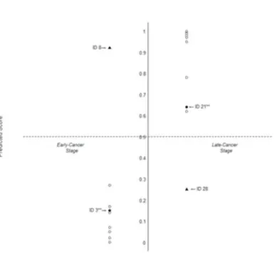
Figure 3.2. Prediction on the thirty patients’ cancer stage with predicted score (Patient ID 3, ID 8, ID21 and ID 28 were predicted incorrectly with DT only; owing to GAS3 and GAS6 employed in TLRM, the predictions for patient ID 3 and ID 21 of the incorrect predictions were being corrected.)
With this pre-classification, patient’s PS for late-cancer stage was calculated with the patient’s significant risk factors, GAS3 and GAS6 which were as large as 1.52 and 0.52, respectively. Since TLRM showed negative effects of GAS3 and GAS6 for late-cancer stage (Table 3.1), the patient’s PS for late-cancer stage was low as 0.02. With TLRM this patient was predicted as early-cancer stage and in actuality this patient was clinically in the early-cancer stage.
3.2. Assessment of TLRM
To assess TLRM, the patient’s cancer stage was predicted based on the patient’s PS. Figure 3.2 shows the prediction for thirty patients’ cancer stages with PSs obtained by the suggesting TLRM Equation (3.1), where a patient with a PS greater than 0.5 was predicted as the late-cancer stage.
Among the twelve patients diagnosed clinically as early-cancer stage (Table 3.3 & Figure 3.2), six, four, and two patients were classified into the subgroup of low risk, in-between risk and high risk, respectively; with TLRM all were correctly predicted as ‘early-cancer stage’ except ID 8. Similarly, among the eighteen patients diagnosed clinically as late-cancer stage, one, one, and sixteen patients were classified into the subgroup of low risk, in-between risk and high risk, respectively; with TLRM all were correctly predicted as ‘late-cancer stage’ except ID 28.
Predictions on the patients pre-classified into high- and low-risk for late-cancer stage were perfectly matched with their clinical diagnoses, except patient ID 8, while patient ID 28 predicted incorrectly, was the one pre-classified into the in-between risk. Owing to the continuous predictors employed in TLRM, ID 3 and ID 21 of being assigned high- and low- risk were correctly predicted as early-cancer and late-cancer stage, respectively, which resulted in the improvement of performance comparing to
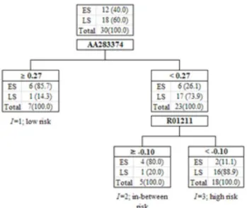
Figure 3.3. Result of CART performed with 28 genes in SIG (The optimal split-values for AA283374 and R01211 are 0.27 and
−0.10, respectively. The number of patients is written in the corresponding leaf, and % is in parenthesis.)
DT (Figure 3.2). The performance of the predictions for all of the samples was evaluated by a cross- validation technique; briefly, one withheld a sample, built a TLRM based only on the remaining samples, and predicted the class of the withheld sample. The process was repeated for each sample, and the cumulative error rate was calculated. The result showed an accuracy of 83.3% for all of the patients while the classification using DT only showed an accuracy of 80.0%.
3.3. Comparison to the method of CART(classification and regression tree)
Using CART algorithm (Breiman et al., 1984) suggested by Breiman, we searched for all possible genes and all possible copy-number change values in order to find the best split that separates the set of samples (patients) into two parts with maximum homogeneity. The process was then repeated for each of the resulting patients fragments. Maximum homogeneity of child nodes is defined by the impurity function i(t). Gini splitting rule is most broadly used for impurity. It uses the following impurity function i(t) as i(t) = 1−∑
kp(k|t)2, where k is an index of class 1, . . . , K, and p(k|t) is conditional probability of class k provided we are in node t.
At each node, CART solves the following maximization problem:
arg max
xj ≤S(xj ), j=1,2,...,M
[i(tp)− Pr[i(tr)]− Pl[i(tl)]] ,
where trand tlare right and left child nodes of the parent node tp, and Prand Plare probabilities of right and left nodes for any of the possible splits xjsuch that xj≤ S(xj) and the best splitting value S(xj) of the variable xj.
For the comparison to TLRM, CART was performed with copy-number changes of the 28 genes in SIG of the CMRC data; the selected, interacting genes were ID AA283374 and R01211as shown in Figure 3.3. Their splitting values were 0.27 and−0.10, respectively.
Cross-validation for evaluation was performed using leave-one-out cross-validation technique and
the accuracy was shown to be 57% which is poor in comparison to our method of using GASs, the weighted sums of the copy-number changes. For the comparison of classification method that utilizes patients’ GASs instead of individual genes’ copy-number changes, CART was performed using GASs and it showed an accuracy of 80.0% in the evaluation for all patients.
4. Discussion
This article shows a statistical strategy that makes it possible to predict patients’ classes with high performance from genes that show a high frequency of alteration in copy-number changes between different classes in cDNA microarray-based CGH; high- and low-risk patients were investigated by pre-classifying homogeneous patients based on the copy-number changes of the selected genes and predicted with increased performance owing to the continuous predictor of patients’ classes employed in the model.
Since cDNA microarray-based CGH data included low-intensity spots, a statistical strategy to detect subtle differences between the two cancer stages was needed. For this purpose, firstly genes with relatively large variations between genes compared to total variations were collected after within- print tip, intensity-dependent normalization of the data. Of those selected genes, genes displaying a high frequency of alteration in either the early- or late-cancer stage were selected after categorizing the genes into alteration/non-alteration using a defined criterion, +0.3 and−0.3 for log2 of copy- changes. SIG was determined according to two parameters that could distinguish cancer stages.
Common latent factors (named GASs) were obtained by utilizing factor analysis to relate patients’
genetic information to the patients’ cancer classification.
A DT was utilized to pre-classify homogeneous patients based on the patients’ GASs by dealing with interactions between GASs. The patient’s index that pre-classified homogeneous patients was created in this utilization of DT. The suggesting TLRM employed the patient’s index and GASs that can be used to calculate a continuous risk score for a given patient and identify patients’ cancer classification in the logistic regression that improves its performance compared to logistic regression or DT only; this made it possible to pre-classify homogeneous patients based on the patients’ genetic alteration scores that use a patient’s index; this also made it possible to rank the risk score for each subgroup pre-classified and investigate high- and low-risk patients on which predictions could be made with the improved performance due to the incorporation of continuous risk factor(s) in the model.
With TLRM thirty patients were pre-classified into three subgroups of low risk, in-between risk, and high risk. All of the patients pre-classified into low- and high-risk were correctly predicted as early- and late-cancer stage, respectively, except one patient.
Four patients were predicted incorrectly using DT only while two predictions of the four predictions were being corrected with TLRM, which improved its accuracy when compared to DT.
Comparing to CART utilizing individual genes’ copy-number changes or patients’ GASs, TLRM showed a superior performance. Accuracies for TLRM, DT, CART, and CART that utilized in- dividual genes’ copy-number changes were 83.3%, 80%, 80% and 56.7%, respectively which were evaluated through a cross-validation technique.
In addition, TLRM provided insight into the prediction for the patient’s risk probability and each gene’s impact on the risk factor(s) for cancer classification.
When the sample size is large we can expect a superior performance of the suggesting model and
the application of bootstrapping or methods of ensemble could be a possible solution to the problem of overcoming the small size of samples.
References
Breiman, L., Friedman, J. H., Olshen, R. A. and Stone, C. J. (1984). Classification and Regression Tree, Champmans & Hall.
Cheng, C., Kimmel, R., Neiman, P. and Zhao, L. (2003). Array rank order regression analysis for the detection of gene copy-number changes in human cancer, Genomics, 82, 122–129.
Inoue, H., Matsuyama, A., Mimori, K., Ueo, H. and Mori, M. (2002). Prognostic score of Gastric Cancer Determined by cDNA Microarray, Clinical Cancer Research, 8, 3475–3479.
Kawaguchi, K., Honda, M., Yamashita, T., Shirota, Y. and Kaneco, S. (2005). Differential gene alteration among hepatoma cell lines demonstrated by cDNA microarray-based comparative genomic hybridiza- tion, Biochemical and Biophysical Research Communications, 329, 370–380.
Kim, M. (2009). Reproducible gene selection algorithm with random effect model in cDNA microarray-based CGH data, Expert Systems with Applications, 36, 11589–11594.
Kim, M. and Chung, H. C. (2009). Standardized genetic alteration score and predicted score for predicting recurrence status of gastric cancer, Journal of Cancer Research and Clinical Oncology, 135, 1501–
1512.
Liu, K. H. and Huang, D. S. (2008). Cancer classification using Rotation Forest, Computers in Biology and Medicine, 38, 601–610.
Mestre-Escorihuela, C., Rubio-Moscardo, F., Richter, J. A., Siebert, R., Climent, J., Fresquet, V., Beltran, E., Agirre, X., Marugan, I., Mar´ın, M., Rosenwald, A., Sugimoto, K. J., Wheat, L. M., Karran, E. L., Garc´ıa, J. F., Sanchez, L., Prosper, F., Staudt, L. M., Pinkel, D., Dyer, M. J. and Martinez-Climent, J. A. (2007).
Homozygous deletions localize novel tumor suppressor gene in B-cell lymphoma, Blood, 109, 271–280.
Park, C. H., Jeong, H. J., Choi, Y. H., Kim, S. C., Jeong, H. C., Park, K. H., Lee, G. E., Kim, T. S., Yang, S. W., Ahn, S. W., Kim, Y. S., Rha, S. Y. and Chung, H. C. (2006). Systematic analysis of cDNA microarray-based CGH, International Journal of Molecular Medicine, 17, 261–267.
Pinkel, D. and Albertson, D. G. (2005). Array comparative genomic hybridization and its applications in cancer, Nature Genetics, 37, S11–S17.
Squire, J. A., Pei, J., Marrano, P., Beheshti, B., Bayani, J., Lim, G., Moldovan, L. and Zielenska, M. (2003).
High-resolution mapping of amplifications and deletions in pediatric osteosarcoma by use of CGH analysis of cDNA microarrays, Genes Chromosomes and Cancer, 38, 215–225.
Yang, S. H., Seo, M. Y., Jeong, H. A., Jeung, H. C., Shin, J., Kim, S. C., Noh, S. H., Chung, H. C. and Rha, S.
Y. (2005). Gene copy number change events at chromosome 20 and their association with recurrence in gastric cancer patients, Clinical Cancer Research, 11, 612–620.
Yang, Y. H., Dudoit, S., Luu, P., Lin, D., Peng, V., Ngai, J. and Speed, T. (2002). Normalization for cDNA microarray data: A robust composite method addressing single and multiple slide systematic variation, Nucleic Acids Research, 30, e15.