†
*
**
This paper was supported by Research Fund, Kumoh National Institute of Technology.
Seunghyun Park, Master‘s Student, Dept. of Computer Engineering, Kumoh National Institute of Technology.
[email protected]
Byoung-Woo Oh, Professor, Dept. of Computer Engineering, Kumoh National Institute of Technology. [email protected] (Corresponding Author)
A Parallel Processing Technique for Large Spatial Data
대용량 공간 데이터를 위한 병렬 처리 기법
†Seunghyun Park ․ Byoung-Woo Oh
박승현* ․ 오병우**
요 약 그래픽 처리 장치(GPU)는 내부에 대량의 산술 논리 연산 장치(ALU)를 보유하고 있다. 대량의 ALU는 병렬 처 리를 위해 이용될 수 있으므로, GPU는 효율적인 데이터 처리를 제공한다. 공간 데이터를 지도상에 표현하기 위하여 지 리학적 좌표가 필요하다. 좌표들은 측지경도와 측지위도의 형태로 저장된다. 데카르트 좌표계로 구성된 지도를 표현하 기 위하여 측지경도와 측지위도는 국제 횡단 메르카토르 좌표계(UTM)로 전환돼야 한다. 좌표계 변환 과정과 변환된 좌 표를 화면상에 표현하기 위한 렌더링 과정은 복잡한 부동 소수점 계산이 필요하다. 본 논문에서는 성능 향상을 위해 GPU를 활용한 좌표변환 과정과 렌더링 과정을 병렬적으로 처리하는 기법을 제안한다. 대용량 공간 데이터는 파일로 디 스크 내에 저장된다. 대용량 공간 데이터를 효율적으로 처리하기 위하여 공간 데이터 파일들을 하나의 대용량 파일로 병합하고 Memory Mapped File 기법을 활용하여 파일에 접근하는 기법을 제안한다. 본 논문에서는 TIGER/Line 데이 터를 활용하여 747,302,971개의 점으로 구성된 공간 데이터의 좌표 변환 및 렌더링 처리 과정을 GPU를 활용하여 병렬 로 수행하는 연구를 진행한다. CPU를 이용하여 좌표변환 과정 결과와 렌더링 처리 과정 결과를 비교하여 속도 향상 정 도에 대한 결과를 제시한다.
키워드 : GPU, CUDA, Memory Mapped File, 병렬 처리, 공간 데이터
Abstract Graphical processing unit (GPU) contains many arithmetic logic units (ALUs). Because many ALUs can be exploited to process parallel processing, GPU provides efficient data processing. The spatial data require many geographic coordinates to represent the shape of them in a map. The coordinates are usually stored as geodetic longitude and latitude. To display a map in 2-dimensional Cartesian coordinate system, the geodetic longitude and latitude should be converted to the Universal Transverse Mercator (UTM) coordinate system. The conversion to the other coordinate system and the rendering process to represent the converted coordinates to screen use complex floating-point computations. In this paper, we propose a parallel processing technique that processes the conversion and the rendering using the GPU to improve the performance. Large spatial data is stored in the disk on files. To process the large amount of spatial data efficiently, we propose a technique that merges the spatial data files to a large file and access the file with the method of memory mapped file. We implement the proposed technique and perform the experiment with the 747,302,971 points of the TIGER/Line spatial data. The result of the experiment is that the conversion time for the coordinate systems with the GPU is 30.16 times faster than the CPU only method and the rendering time is 80.40 times faster than the CPU.
Keywords : GPU, CUDA, Memory Mapped File, Parallel processing, Spatial Data
1. 서 론
The Graphical Processing Unit(GPU) is originally used for processing computer graphics. To assure rendering beautiful graphic effect, the GPU has a lot of arithmetic logic units (ALUs). The number of the GPU’s ALU is larger than the CPU’s. This makes the
GPU operate floating point more rapid than the CPU.
Compare with the GPU and the CPU computing speed, the GPU is superior to the CPU’s computing speed.
Therefore, the GPU can be used to process computations
because of the GPU’s overwhelming ability compared
with the CPU. The GPU’s cores are constructed in
parallel. It is possible to be used to improve performance,
which processes same calculation with many data.
There are many researches about parallel processing using the GPU in many areas. In algorithm area, there are many researches about sorting algorithms in parallel [1,2,3]. In multimedia area, researches are being preceded for image processing and coding moving pictures[4,5,6,7,8].
Spatial data have been widely used as the location becomes important in the mobile environment. There are many studies to process spatial data efficiently.
When users process spatial data, they want to represent spatial data onto a map. It takes much time to process spatial data because they usually contain a large amount of coordinates which are necessary to compute the geometry calculation. It is inefficient to process spatial data only using the CPU. Thus, there are attempts to apply parallel processing of spatial data not only using the CPU but also using the GPU[9,10,11]. Lee[11]
tried to use the GPU to calculate graphics transform operations, such as rotate, scale, and translate. As a result of Lee[11], it takes much time to transfer the result of the graphics transform operations from the GPU to the CPU. In order to reduce the transferring time for the result, we propose a technique that renders the calculated coordinates in parallel way and transfers the final rendered bitmap to the CPU.
In this paper, we propose a parallel processing technique for large spatial data. It deals with the large file that stores spatial data bigger than 4GB. Many original spatial data files are merged to three files:
spatial record file, part file, and point file. The spatial record file and part file are smaller than 4GB, but the point file is very large. The size of a point file for the experiment is 11GB. The logical limit of the size is 16EiB in the 64-bit operating system. If the point file is very large, it is hard to load whole spatial data into main memory. We exploit the memory mapped file provided by the Microsoft Windows operating system to access the very large point file efficiently.
The memory mapped file provides access a file as a way of a memory access. Memory mapped file loads a part, named as view, of a file to the main memory.
This process is useful to access large spatial data sequentially. Some studies exploit the memory mapped file to share data[12]. The proposed technique loads
the large spatial data with the memory mapped file and processes the loaded spatial data in parallel way.
The result of the parallel process is rendered onto a bitmap in parallel way again.
This paper is organized as follows. Chapter 2 in- troduces CUDA and memory mapped file. Chapter 3 describes the proposed technique for processing large spatial data with CUDA. Chapter 4 reports the result of the experiment. Finally, chapter 5 presents con- clusion and future work.
2. Related Works
2.1 CUDA
NVIDIA developed computing unified device archi- tecture (CUDA) for general purpose usage of the GPU[13]. After introducing CUDA, researchers have applied GPU technology in many areas. The researchers can easily process a large amount of data efficiently by utilizing parallelism of the GPU. CUDA’s codes are written by C language and exploited in the GPU.
CUDA accesses to distinct command and memory of the GPU. CUDA is provided by NVIDIA Geforce ser- ies the GPU.
CUDA consists of threads, blocks which are set of thread and Grids which are sets of block. Each kernel function makes grid for parallel processing. The Grid makes one or two dimensional block. Block makes three dimensional threads and allocates calculation.
CUDA usually uses three memories which are local memory, shared memory, global memory. Each thread has own local memory. Each block has shared memory which is for sharing data between threads which are in the block.
CUDA provides kernel functions which can be exe- cuted on many GPU cores in parallel. In the kernel function, CUDA sets the number of blocks and threads by using symbols; “<<<”, “>>>”. Symbol “>>>”
makes threads which are applied to operation. Symbol
“<<<” determines that the number of blocks are used
for operation. Total numbers of threads for operation
are calculated at the number of blocks times the num-
ber of threads per each block. CUDA provides varia-
bles for operation. Threads which are in a block have
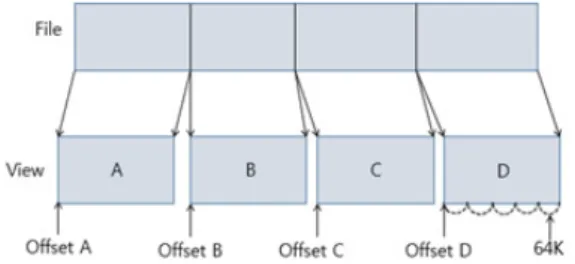
Figure 1. Example of accessing a memory mapped file own variable which is called threadIDX. By setting di- mension of thread, threadIDX can have values of x, y and z. Variable blockIDX which is built in variable in CUDA identifies a block in Grid. Variable blockdim identifies that blocks are set to one or two dimension.
The variables can be accessed in kernel function. In order to process data on the GPU, CUDA introduces kernel functions which are built in CUDA. Kernel function “cudaMalloc()” function allocates memory on the GPU memory. For transmitting data between CPU memory and GPU memory, “cudaMemcpy()” function is used.
2.2 Memory Mapped File
Memory Mapped File (MMF) which is provided by Operating System is a way to handle files. MMF is used to handle large files. MMF maps memories of parts of file to virtual memory on process. MMF can be shared with several processes. Blocks of file are connected with Pages in process. MMF processes I/O performance by approaching addresses of virtual mem- ory directly. Data are not changed simultaneously on processing MMF. Data are changed when memory frees Pages or MMF is closed. Because approaching memory directly, it is efficient for MMF to handle large files. When data of files are changed, whole files are allocated to main memory and saved again. It takes much time to handle files. Though, MMF loads part of a file into main memory without loading whole files.
It can improve performance.
Figure 1 shows a block diagram of MMF. In order to use MMF, users create Views which can be entire file or part of the file. MMF handles large file by using Views. Views consist of Pages. Pages are constructed at 64Kb. Users make views at 64Kb when utilizing
Views. The views are allocated to virtual memory on process. When we have to change data on file, we find location of the data by offset of views. For example, we change data which are in View C area. We find offset of View C. View C is loaded into main memory.
After change the data of View C, changed data are maintained in file which is in disk. Without data of View C, other data are not changed and maintained in disk. This process is a benefit of MMF. Therefore, MMF has a benefit for processing spatial data. Files which consist of spatial data are very large. When we scale spatial data in shape file, spatial data in shape file are changed. It takes much time to load shape file to memory and saved to disk. Though, MMF loads data which are had to change to memory and reduces processing time.
3. Technique for processing large spatial data
We propose a parallel processing technique for large spatial data. The main idea of the proposed technique consists of two parts: using memory mapped file for large spatial data and using the GPU to calculate the coordinates of the spatial data and to render the result of the calculation.
3.1 File and Data Structure
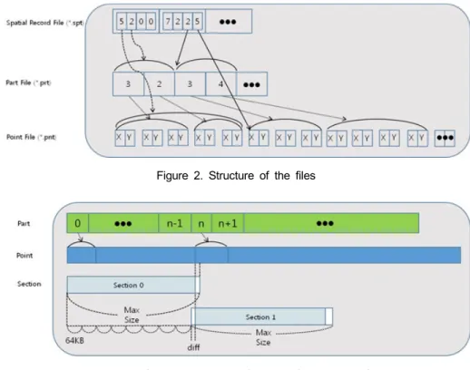
There are several kinds of types for spatial data, such as point, polyline, polygon, etc. In this paper, we deal with the polyline data type. A polyline consists of one or more parts. The part of the polyline consists of one or more line segments with points. Figure 2 shows the structure of the three files: spatial record file (*.spt), part file (*.prt), and point file (*.pnt).
The spatial record file consists of 4 attributes: the number of points, the number of parts, the starting in- dex of the part, and the starting index of the point.
In Figure 2, the first record in the spatial record file represents that it has 5 points and 2 parts. The start index of the part file is 0.
The start index of the point file is 0. The part file
has only the number of points. In Figure 2, the first
part in the part file has 3 points. The point file has
Figure 2. Structure of the files
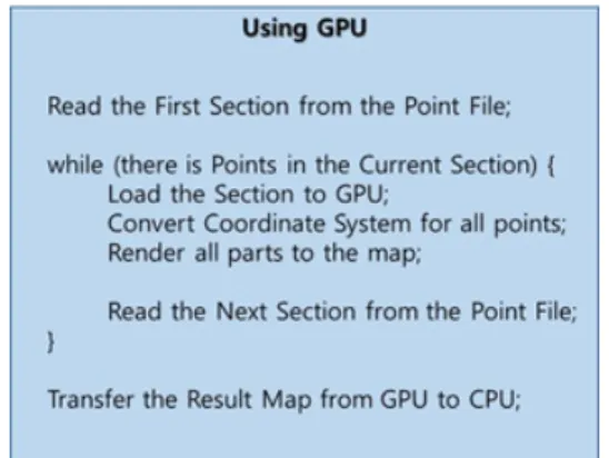
Figure 3. Section in-memory Structure for the point file
x and y coordinates for each point.
For processing spatial data on GPU, spatial data should be allocated to memory in the GPU. According to the limit of the main memory size and GPU memory size, large point file cannot be allocated to main memory and GPU memory. Figure 3 shows the memory structure to process spatial data. The part structure is loaded from the part file (*.prt) onto the main memory and the GPU memory at the same time.
Since the point is very large file, it could not be loaded onto the memory in the whole file. In order to load onto the memory, it should be divided by section. The max size of the section is decided by the size of the memory in the GPU. We use the half size of the GPU’s memory size as the max size.
Because the section size cannot exceed the max size, the section 0 is assigned the parts from 0 to n-1. Notice that the rectangle (white box) which is located at the right and is not filled with color in Figure 3 contains nothing in section 0. The section 1 has parts from n as shown in Figure 3. The starting offset of the first point of the section 1 is expected to be the starting offset of the first point of the nth part. There is
restriction of using memory mapped file. A memory mapped view of a file aligned to 64KB boundaries.
When the process read the section 1 from the point file, the start offset should be adjusted to the unit of 64KB. The left-side white rectangle area of the section 1 represents the adjustment in Figure 3. The section loaded from the point file is transferred to the GPU memory.
There are three functions are used to manage the memory mapped file in the Microsoft Windows operating system, such as CreateFile(), and CreateFile Mapping(), and MapViewOfFile() function. The Create File() function opens the point file with parameters, such as GENERIC_READ, OPEN_EXISTING, FILE_FLAG_
SEQUENTIAL_SCAN. The CreateFileMapping() function
prepares the memory mapped file with parameter
PAGE_READONLY. The MapViewOfFile() function
returns a pointer to the memory address. The section
data structure stores high, low, and diff attributes to
be used to call the MapViewOfFile() function. The high
attribute is used to set the high-order DWORD of the
file offset where the view begins. The low attribute
is the low-order DWORD. The diff is the start offset
Figure 4. Algorithm of Processing Sections Using GPU of the actual point. It’s presented as the left-side white rectangle area of the section 1 in Figure 3.
Memory is allocated in the GPU with cudaMalloc() function before processing the section. The size of the memory allocated in the GPU is represented as the max size in Figure 3.
Once the memory is allocated in the GPU, then the memory is reused for every section to load point data.
3.2 Processing Section
Since the spatial data are usually large, it should be divided into smaller part to fit in the memory size.
In this paper, we divide the point file into sections.
The section is corresponding to the view of the memo- ry mapped file. For processing large spatial data effi- ciently by using memory mapped file, there are two methods; merging files and making section. In order to improve processing time, it is efficient to merge original spatial data files into a file. The limit of the file size is 4GB in shape file format (*.shp) which is the de-facto standard to share spatial data. For exam- ple, the sum of the sizes of the shape files which con- sist of whole edges (all lines theme) of the TIGER/Line shape file is bigger than 4GB. Loading each shape files to memory is not efficient. We merge the shape files and convert to three files as described in the section A.
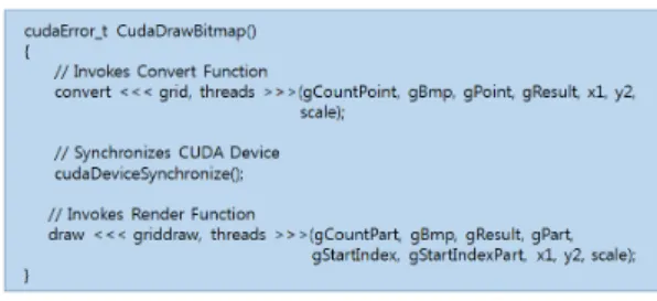
Algorithm of processing sections are shown in Figure 4.
The sections are read sequentially from the point file and loaded onto the main memory. After reading a sec- tion, the section should be transferred to the GPU.
The cudaMemcpy() function is used to load the point
of the section onto the GPU memory. The TIGER/Line data use the North America Datum (NAD83). To dis- play a map in 2-dimensional Cartesian coordinate sys- tem, the point loaded to the GPU should be converted from the geodetic coordinate system to the Universal Transverse Mercator (UTM) coordinate system. The conversion includes graphics transform such as scale and translation, in this paper. The converted coordinate is rendered to the bitmap. The conversion and the ren- dering are processed in parallel way to increase the performance using CUDA.
The last step is the transferring the result bitmap from GPU to CPU by calling CudaGetBitmapFromGPU() function. The bitmap is the device independent bitmap (DIB). It is described in the next section.
3.3 Using CUDA
There are several functions designed for using CUDA in this paper. The CudaInit() function calls the cudaGetDeviceProperties() to get the total global mem- ory in the GPU. The CudaAllocData() function calls the cudaMalloc() function to allocate the point data and the result of the coordinate conversion. CudaLoadPart DataFromCPU() function allocates and copies the part data. CudaSetBitmapFromCPU() function allocates the device independent bitmap (DIB) to be used to render spatial shape and copies the DIB from the CPU to the allocated DIB. The DIB is a data structure for the Windows graphics. It contains the device independent pixel array for bitmap. The size of the bitmap is set to 1920 x 1080. The DIB is created by calling the CreateDIBSection() function and is selected to the buf- fer device context (DC) as the bitmap object. These functions are called when the document is loaded be- fore processing sections.
The CudaTransferSectionPointDataToGPU() func- tion loads the point data to the memory already allo- cated by the CudaAllocData() function. The main func- tion is CudaDrawBitmap(). It invokes the CUDA glob- al functions, such as convert() and render(). Figure 5 shows the pseudo code of the CudaDrawBitmap() function.
The convert() function is executed in parallel and
converts the coordinate system. Figure 6 shows the
Figure 5. Main Function for Drawing a Map in Parallel
Figure 6. Convert Function for the Coordinate System
Figure 7. Render Function for Drawing Lines onto the DIB
pseudo code of the convert() function.
Before draw DIB in parallel, we should translate co- ordinate in parallel. Original coordinates consist of NAD83 coordinates. It is not useful to express spatial data on the flat screen. We translate NAD83 coordinate to TM coordinate. In order to translate coordinates in parallel, GPU calls convert() function. Execution con- figuration of function consists of two variables; grid and threads. Variable “grid” means the number of blocks which are in CUDA cores and “threads” means the number of threads which are in a block.
Converted points are drawn on the DIB by calling render() function in parallel. Figure 7 shows the pseudo code of the render() function.
The render() function uses similar execution config- uration which is used for convert() function. The con- vert() function uses the number of points and the ren-
der() function uses the number of parts. In order to draw a map, GPU should put pixels and draw lines on DIB in parallel. There are two CUDA device func- tions; __device__ DrawLine() and __device__ PutPixel().
These functions are invoked by the CudaDrawBitmap() function. By Calling these functions, we can draw a map in parallel.
After drawing a map, CUDAGetBitmapFromGPU() function is called. GPU transfers bitmap from GPU memory to CPU memory. CPU transfers points of next section and bitmap from CPU memory to GPU memory. These processes continue until points of last section and bitmap are transferred and drawn on GPU.
Finally, a map is shown on screen after drawing points of last section on DIB in GPU.
4. Experiment and Result
All experiments are performed on a machine Microsoft Windows 7 with an Intel® Core™ i7-3770 CPU running at 3.40GHz and 16GB of memory. It is equipped with an NVIDIA GeForce GTX Titan Black graphic card. It has 2,880 CUDA cores. Each CUDA core contains arithmetic logic unit(ALU) for calculat- ing floating point. The memory size of the graphic cars is 6GB. It is used to loading data for CUDA or graphic operations. Memory interface width of the graphic card is 384-bit and memory bandwidth is 336GB per second. We implement the test system with the CUDA SDK version 6.5. The storage for the spatial data is the 256GB SSD.
4.1 Data Set
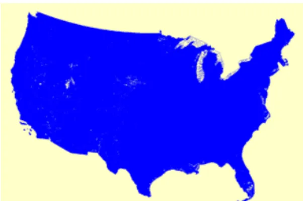
The data set for experiment is a set of the edges of United States of America whose layer type is all lines in the TIGER/Line data. The Alaska and Hawaii states are excluded only for the shape of the display.
The Tiger/Line data files contain geographic features such as roads, rivers, zip codes, political boundaries, legal and statistical geographic areas, etc. The U.S.
Census Bureau developed the TIGER/Line data and
provides files on its website[14]. Figure 8 shows whole
data set. There are 68,967,233 spatial records and
747,302,971 points in the data set.
Figure 8. Edges Data set of the TIGER/Line data
Figure 9. Algorithm of Processing Sections Using CPU for Comparison
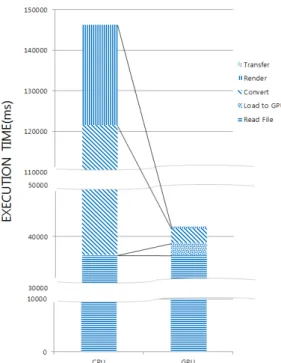
Table 1. Result of the Experiments
CPU/GPU Read File Load to GPU Convert Render Transfer Total
CPU 36,386.62ms - 85,186.81ms 24,679.70ms - 146,253.13ms
GPU 36,386.62ms 2,324.09ms 2,824.79ms 305.52ms 1.46ms 41,842.17ms
4.2 Implementing the System for the Experiment In order to implement the experiment, several shape files were merged into one file. Original shape files contained whole edges of each state. In order to show whole edges of the United States of States, we merged several shape files into one shape file. We divided edges 4 areas such as western, central, south-eastern and eastern edges because of the limit size of shape file. We made spt, prt, and pnt files for showing whole edges of United States of America. Figure 8 shows whole edges of United States of America after merging into a file. In order to gather reliable result, we exe- cuted experiment 1,000 times. Figure 9 shows the algo- rithm of processing section using CPU for comparison with the GPU usage.
4.3 Result of the Experiment
To compare the performance, experiment was exe- cuted on CPU and GPU. Translating coordinates and drawing a map were executed on CPU, and then exe- cuted on GPU, and total execution times were compared.
Total time was gathered by adding Read File, Load to GPU, Convert, Render, Transfer DIB times. Table 1 shows the results for total execution time.
The execution times on CPU were gathered at 146,253.13 ms. The gap of execution time between CPU and GPU arose at the Convert time and Draw time. The Convert time on CPU took 85,186.81ms. In contrast, the Convert time on GPU took 2,824.79ms. The result means that the conversion of coordinates of points on GPU is 30.16 times faster than CPU. The gap of the Render time is much bigger than the Convert time. The Render time on CPU took 24,679.70ms.
The Render time on GPU took 305.52ms and 1.46ms to transfer the result DIB. The rendering time on GPU is 80.40 times faster than CPU. Those two gaps of re- sult made performance different.
As can be seen in Figure 10, processing large spatial data on GPU is much faster than executed on CPU.
The gap of performance time arose mainly in the Convert time and the Render time. The reason why GPU is faster than CPU is that translating coordinates and drawing a map was executed in parallel. When drawing a map on GPU, putting pixels and drawing lines were processed in parallel on DIB. Though, costs of drawing a map on CPU increased because putting pixels and drawing lines sequentially. This could re- duce much performance time than executing on CPU.
The experiment showed that processing spatial data on GPU improves performance 3.50 times faster com- pared to processing on CPU.
5. Conclusion
This paper proposed the parallel processing techni-
Figure 10. Comparison of the execution time between CPU and GPU
que for large spatial data by using memory mapped file and GPU. It achieves high speed by handling large volume of file efficiently and applying parallelism of GPU on main processes. In general, volumes of spatial data are large. According to limit size of memory, this occurred memory problem. In order to solve this prob- lem this arose when processing large spatial data, this paper applies memory mapped file to processing large spatial data. Files which include whole edges of the United States of America are up to 11GB. These files can’t be loaded in main memory. Therefore, this paper makes intersection to handle those files. Spatial records of whole spatial data divided into several sections.
Sections can be loaded in main memory. In order to improve performance, this paper applies technique.
Technique is that preloads next section while present section is processed. Another way to improve perform- ance is to use GPU for parallelism. In order to process spatial data in parallel, points of spatial data and bit- map are copied to GPU memory. In order to improve performance, GPU memory preloads parts and points start index. On GPU, coordinates of spatial data are translated in parallel. For drawing a map, it is needed
to put pixels and draw lines. This paper puts pixels and draws lines on DIB in parallel. CUDA kernel func- tions make them available. Those processes enhance performance. After drawing a map on GPU, Bitmaps which include map are copied to main memory.
Proposed two ways to process large spatial data enhan- ces performance. In order to prove that proposed meth- ods are efficient, the execution time is compared with the Convert time and the Render time between CPU and GPU. With respect to performance time, the Convert time and the Render time which executed on GPU are much faster than executed on CPU. The pro- posed technique enhances the performance 350%.
Our future works could focus on combining the tech- nique with the distributed system using Hadoop.
References