A Comprehensive Analysis of the End-to-End Delay for Wireless Multimedia Sensor Networks

(1)

2456

A Comprehensive Analysis of the End-to-End Delay for Wireless

Multimedia Sensor Networks

**Nasim Abbas* and Fengqi Yu**

†

Abstract

– Wireless multimedia sensor networks (WMSNs) require real-time quality-of-service (QoS) guarantees to be provided by the network. The end-to-end delay is very critical metric for QoS guarantees in WMSNs. In WMSNs, due to the transmission errors incurred over wireless channels, it is difficult to obtain reliable delivery of data in conjunction with low end-to-end delay. In order to improve the end-to-end delay performance, the system has to drop few packets during network congestion. In this article, our proposal is based on optimization of end-to end delay for WMSNs. We optimize end-to-end delay constraint by assuming that each packet is allowed fixed number of retransmissions. To optimize the end-to-end delay, first, we compute the performance measures of the system, such as end-to-end delay and reliability for different network topologies (e.g., linear topology, tree topology) and against different choices of system parameters (e.g., data rate, number of nodes, number of retransmissions). Second, we study the impact of the end-to-end delay and packet delivery ratio on indoor and outdoor environments in WMSNs. All scenarios are simulated with multiple run-times by using network simulator-2 (NS-2) and results are evaluated and discussed.

Keywords:

Wireless sensor networks, End-to-end delay, Indoor environment, Outdoor environment, Reliability.

1. Introduction

Recent advances in micro-electro-mechanical systems (MEMS) technology, embedded computing, and wireless communications has motivated the development of wireless sensor networks (WSNs) [1-2]. Each sensor node can be equipped with inexpensive hardware such as microphones and CMOS cameras. This fostered the development of wireless multimedia sensor networks (WMSNs) [3-4]. WMSNs have been widely applied to mobile learning [5], healthcare [6], video surveillance [7], and biomedical imaging [8]. Numerous studies have been carried out in recent years on the physical layer [9], the media access control (MAC) layer [10], the network layer [11], and the transport layer [12-13] in WMSNs.

Nowadays, there has been extensive research in solving WMSNs issues. There are numerous issues that must be addressed such as lack of fixed infrastructure, high variable delays, limited bandwidth, shared channel, high packet loss rate, and mobility in WMSNs [14-15]. However, main issue of providing efficient quality of service (QoS) guarantees for real-time transmission in WMSNs is still open and largely unexplored. The end-to-end delay is very

important QoS metric for WMSNs and WMSNs need end-to-end delay guarantee for delay sensitive data. Compared to the single-hop transmission, the analysis of end-to-end delay in multi-hop WMSNs is more challenging due to delay accumulation at each hop. Many factors can impact the end-to-end delay in multi-hop WMSNs, such as routing algorithm, network topology, traffic model, and data scheduling [16]. Therefore, it is very significant to investigate the comprehensive analysis of end-to-end delay in multi-hop WMSNs.

WMSNs require reliable and timely communication of data. However, radio transmission errors in wireless channel make it hard to get these qualities at the same time. To obtain balanced reliability and delay performance, system may choose to compromise on its reliability and have nodes discarding few packets forcibly. In order to ensure 100% packet delivery in a fully reliable network, unsuccessful packets will be retransmitted until they are received successfully. The resulting end-to-end delay will be too large and cannot be tolerated by real-time WMSNs applications. In addition, more energy will be required to send the lost packets again. Therefore, it is indispensable to provide WMSNs a balanced guarantee between end-to-end delay and reliability. Otherwise severe distortion will appear in the services and make the users intolerable. In WMSNs, a feasible solution to balance end-to-end delay is to discard the packets after some retransmission attempts. Although, reliability of network is reduced marginally, the end-to-end delay of most of the packets can be greatly reduced. To effectively study the QoS offered by the † Corresponding Author: Shenzhen Institutes of Advanced Technology,

Chinese Academy of Sciences, Shenzhen, China.

University of Chinese Academy of Sciences, Beijing, China. ([email protected])

* Shenzhen Institutes of Advanced Technology, Chinese Academy of Sciences, Shenzhen, China.

University of Chinese Academy of Sciences, Beijing, China. ([email protected])

(2)

WMSNs, it is critical to investigate the importance of end-to-end delay which is the primary focus of this paper.

In this article, we tackle the challenging problem of end-to-end delay analysis in WMSNs. Our approach has many advantages over a fully reliable network. First, network stability is not a problem. If the traffic load is too heavy, few packets will be dropped and eventually the network will become stable. Second, fewer energy is required to retransmit the lost packets that will be discarded ultimately. The end-to-end delay constraint is modeled by assuming that each packet is allowed fixed number of retransmissions. To characterize the end-to-end delay, first, we compute the performance measures of the system, such as reliability and end-to-end delay in different topologies (e.g., linear topology, tree topology) and against different choices of system parameters (e.g., data rate, number of nodes, number of retransmissions). Secondly, we characterize how reliability and end-to-end delay is affected by indoor and outdoor environments in WMSNs. In an outdoor environment, we consider four scenarios, i.e., rural, suburban, urban and dense urban environments. Whereas, in an indoor environment, we consider three scenarios i.e. in-building line-of-sight, factory obstructed, and building obstructed environments.

The remaining of this article is organized as follows. Section 2 provides the related work. Section 3 discusses the description of simulation model. Section 4 gives the experimental results. Section 5 concludes our work.

2. Related work

End-to-end delay analysis is very important in WSNs and has been extensively investigated in literature.

Ahmed et al. [17] present a method to optimize delay in mobile ad-hoc networks for multimedia transmission. They minimize the delay by reducing the disorganized packets and by increasing in-order packet in the buffer. Their technique maintains more number of in-order packets by maximizing available space in the buffer. Moreover, they also present a mathematical relationship of delay, buffer size and packet size. However, their technique is useful only when more data is available and buffer size is small. Wang et al. [18] present an inclusive cross layer framework to investigate end-to-end delay distribution in realistic WSNs. Their proposed framework uses stochastic queuing model to provide probabilistic QoS guarantees. They present a generic framework that can be parameterized for various routing and MAC protocols. However, they don’t consider bursty traffic pattern in their proposed simulation. Yu and Kim [19] derive a scaling law for end-to-end delay analysis in wireless networks. However, they assume that transmission channel is error free, and there is no collision when two nodes transmit simultaneously. However, both of the scenarios are unrealistic.

Rahul vaze [20] uses the idea of transmission capacity to characterize the Throughput-delay-reliability (T-D-R)

analysis in wireless ad-hoc networks. They model delay constraint by considering limited retransmissions for each hop. They optimize number of retransmissions and number of nodes to obtain optimal value to maximize a lower bound on the transmission capacity. Zhang et al. [21] study the analysis between the latency and the energy consumption in a wireless multi-hop network. They use both realistic and unreliable models to provide framework to estimate the delay-energy performance in a linear network. They provide closed-form expression to optimize the parameters in cross-layer design to evaluate the energy-delay performance. Liu et al. [22] investigate the packet drop rate and end-to-end delay performance in WSNs. They propose a heuristic scheme to obtain balanced packet drop rate and consequent cluster head timeline allocations. However, their work is just based on cluster tree topology.

Dong et al. [23] present a comprehensive tradeoff between transport delay and energy consumption in wireless sensor networks under certain reliability conditions. Their proposed protocol jointly reduces network delay and improves the network life time by sending fewer data packets with heavier load and by sending more ACKs with fewer load. Xie and Haenggi [24] use bounded delay packet dropping strategy to evaluate the reliability-delay analysis in a linear wireless network. However, they did not present the dependence of link success probabilities on packets dropping events. Bi et al. [25] optimize retransmission threshold in wireless sensor networks. They focus on calculating the optimal retransmission threshold for multi-hop wireless sensor networks by providing upper and lower limits on number of retransmissions. However, they do not characterize the delay-reliability analysis of WMSNs.

3. Simulation model

3.1 Channel model

We use log-normal shadowing model for our analysis.

0 0 ( ( )[ ] [ ] ) 10 r t d P d dBm P dBm PL d nlog X d s æ ö = - - ç ÷ -è ø (1)

Where PL d

(

0

)

is the measured path loss at reference,

X_s is a normal random variable (in dB) with zero mean,

n is the path-loss exponent, P is the power of the r

received signal, and P is the power of the transmitted t

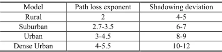
signal. Both n and s are parameters which are dependent on environment and may vary considerably according to communication channel. We deploy WMSNs architecture in variety of communication environments. We consider following deployment options. 1) Indoor deployment: in-building line-of-sight, obstructed factory, and obstructed buildings. 2) Outdoor deployment: rural, urban, suburban

(3)

areas, and dense urban. Typical values of shadowing deviation and path loss exponent for outdoor and indoor environments are mentioned in Table 1 and Table 2.

3.2 Network model

We consider two multi-hop topologies for our simulations: linear topology and tree-based topology

3.2.1. Linear topology

In linear topology, each node (except leave and sink) has two neighbors: one parent and one child node. All sensor nodes can generate and relay traffic. Every node gets packets from its child node and forwards the incoming packets to its parent node to reach the destination.

3.2.2. Tree topology

Tree-based topology is extensively employed in several WMSNs applications. In a tree topology, every parent node has children nodes which are not essentially similar for all of the nodes. All sensor nodes are capable to retrieve multimedia contents and transmit captured information to the destination. All sensor nodes are capable of creating and relaying video traffic.

3.3 System model

Our WMSNs model consists of N number of sensor nodes without any centralized control. Let E=N1,N2,¼,Nn+1 be the end-to-end path from source to destination, where N and Nn+1 represents the source and destination nodes and other Ni s' represents the relay nodes. Each link can be expressed as Ni ®Ni+1. Each link has the following properties. We assume that t is the transmission time taken by each sensor node and P is the transmission failure i

possibility for path Ni ®Ni+1. Let R retransmissions i

are allowed between source and its intended receiver. Therefore, after R + retransmissions, the data packets _i 1 will be discarded by the sender. The probability of a packet being successfully delivered to node Ni+1 is given by

1 1 Ri

i P +

- . Let C represents the number of the packets i

buffered at a sensor node N , which means there are i

1

i

C + packets need to be forwarded.

Let B and L B be the lower and upper bounds of the U

retransmission threshold of node i and d be the delay

constraint. Then, the optimal retransmission thresholds for each node can be given as:

1 1 1 i n R i i max P + =

-å

(

)

1 ( 1) 1 n i i i C R t d = + + £

å

(2)

{

}

, , 1, 2, , L i U i B £R £B RòZ iò ¼n

Each hop delay consists of propagation, transmission, queuing, and processing delays. In this article, we consider queuing delay and transmission delay. Therefore, maximum delay for each hop can be represented as

(

)

(C_i +1) R_i+1 t. The first inequality constraint shows the end-to end delay of last packet should be no more delay constraint d . The second inequality shows that the retransmission thresholds should be bounded in a given interval.

3.4 Framework

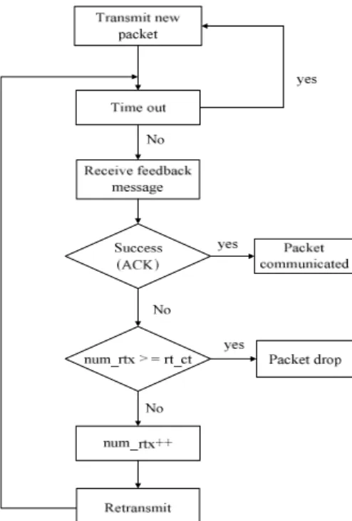
We use stop-and-wait automatic repeat request (ARQ) approach in our end-to-end delay analysis. In SW-ARQ, the receiver sends a NACK to the sender until the packet is successfully received. In the case of a successful packet transmission, the sender will receive an ACK from the receiver. The basic mechanism of SW-ARQ is elaborated in Fig. 1.

The packet sent by the sender can get an error. If the receiver detects an error, it discards the packet and sends a NACK to the sender by informing the sender to resend the lost packet. If the receiver cannot receive the sender's packet, it will not respond to the sender. In order to implement the NACK/ACK mechanism, the sender is equipped with a timer. After a packet is sent, the sender waits for an acknowledgement (ACK or NACK). If no acknowledgement is received during the timeout period, then the packet is resend. Therefore, sender should preserve a copy of the transmitted packet until an ACK is received for that packet. There are two cases when sender cannot receive ACK. One is when ACK is lost, and other is

Table 1. Outdoor environment parameters

Model Path loss exponent Shadowing deviation

Rural 2 4-5

Suburban 2.7-3.5 6-7

Urban 3-4.5 8-9

Dense Urban 4-5.5 10-12

Table 2. Indoor environment parameters

Model Path loss

exponent Shadowing deviation In-building line-of-sight 1.6-1.8 3-4 Obstructed factory 2-3 6.8 Obstructed building 4-6 7-10 Fig. 1. Framework

(4)

when packet itself is lost.

3.5 Sender setup

Fig. 2 represents the sender setup. A sender either sends a new packet or waits for feedback packet. The sender keeps a timeout counter. When sender sends a packet, it starts the timeout counter. If it receives an acknowledge-ment within the specified time period, it sends the next packet. If it does not receive the acknowledgement (Either ACK or NACK) in time, it resends the packet and starts timeout counter again. This approach is suitable for packet loss. However, the receiver may have correctly received the data packet, but the acknowledgement is lost, causing the retransmission of original packet. So the receiver needs to detect and discard these packets. For this purpose, we allocate a unique sequence number to each packet. After receiving the ACK packet, the sender can determine whether the transmission is successful based on the sequence number. The sequence number is initially set to zero and its value is incremented by one each time a new packet is sent. When the sender starts transmission, it assigns a sequence number to each transmitted packet and changes its status to wait for an acknowledgement. When the sender receives an acknowledgment (ACK), it immediately knows that the packet has been successfully transmitted. The sender then informs the buffer to discard the packet and stores the next packet in the buffer. If the sender gets a negative acknowledgment (NACK), it stores the corresponding sequence number in the queue and increments the number of retransmissions. If the sender cannot obtain the packet within the specified retrans-mission threshold, the data packet will be discarded. The

retransmission threshold in the WMSN is very important because if no retransmission limit is set, the delay will increase dramatically. The parameters are shown in Table 3.

3.6 Receiver setup

When the receiver successfully receives a packet, it sends an acknowledgement (ACK) to the sender. The sender receives the ACK and immediately sends the next packet. The receiver gets packet loss information according to the sequence number of the packet. The sequence number field is included in each ACK and NACK packet. If packet loss happens, the receiver sends a NACK to the sender. The information about sequence number is stored in this NACK packet. The packet received field shows that the receiver has accepted a packet from the sender. The sequence number of the received packet is compared with the expected sequence number. If the sequence number matches, the packet is expected, the ACK is sent back to the sender, and the sequence number will be incremented. If sequence number does not match, the sequence number remains same, and packet will be dropped. The Send ACK field shows that receiver has finished processing the packet. It shows that queue has enough space to receive the next packet. It sends an ACK, which contains the next sequence number expected by receiver.

Fig. 2. Sender setup

Fig. 3. Receiver setup

Table 3. Parameters used in reliability mechanism

Symbol Description of parameters

num_rtx The number of retransmissions.

rt_ct The retransmission threshold.

(5)

3.7 Simulation setup

The network simulator-2 (NS-2) [26] is used for all our simulations. Each packet has a size of 1000 bytes. We use following two measures to implement our indoor and outdoor environments.

(1) End-to-End Delay: Time duration from the instant when a packets are originated at the sender node until the time they are received at the destination node.

(2) Packet Delivery ratio: The ratio of the total number of successfully delivered packets to the total number of packets delivered to the destination.

/

r s

PDR=

å

N N (3)

Where Nr shows the number of received packets and Ns shows the number of sent packets.

4. Simulation and Discussion

We consider four scenarios in our simulations. In the first scenario, we measure packet delivery ratio and end-to-end delay in a linear topology in an outdoor environment. In the second scenario, we measure packet delivery ratio and end-to-end delay in a linear topology in an indoor environment. In the third scenario, we measure packet delivery ratio and end-to-end delay in a tree topology in an outdoor environment. In the fourth scenario, we measure packet delivery ratio and end-to-end delay in a tree topology in an indoor environment. Now, we will discuss all four scenarios in details.

4.1 Linear topology with outdoor environment

Fig. 4 shows the relationship between packet delivery rate and number of retransmissions in a linear topology in an outdoor environment. The packet delivery ratio is 93% for rural environment with two retransmissions. The packet delivery ratio reduces to 89%, 84.5%, and 79% for suburban, urban, and dense urban environment respectively with two retransmissions. The simulation results verify that

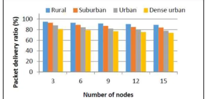
higher number of retransmissions result in higher packet delivery ratio. Fig. 5 represents the relationship between the end-to-end delay and number of retransmissions in a linear topology in an outdoor environment. The end-to-end delay is 75ms with two retransmissions in a rural environment. The end-to-end delay increases to 100.5ms, 124ms, and 149.5ms with the suburban, urban, and dense urban environment respectively with two retransmissions. We observe that more retransmissions result in higher end-to-end delay in suburban, urban and dense urban environments as compared to rural environment. Fig. 6 shows the relationship between packet delivery ratio and number of nodes in a linear topology in an outdoor environment. The packet delivery ratio approaches to 89% for rural environment with 15 nodes. The packet delivery ratio drops to 84%, 78%, and 74% with suburban, urban, and dense urban environment respectively. When number

Fig. 4. Packet delivery ratio vs. number of retransmissions

in a linear topology in an outdoor environment

Fig. 5. End-to-end delay vs. number of retransmissions in a

linear topology in an outdoor environment.

Fig. 6. Packet delivery ratio vs. number of nodes in a linear

topology in an outdoor environment

Fig. 7. End-to-end delay vs. number of nodes in a linear

(6)

of nodes increases, more packets are dropped because specific packet has to go through more obstacles than the less number of nodes.

Fig. 7 represents the end-to-end delay with respect to number of nodes in a linear topology in an outdoor environment. The end-to-end delay is 190ms for rural environment with 15 nodes. The end-to-end delay increases to 235ms, 279ms, and 310 for suburban, urban, and dense urban environment respectively with 15 nodes. Therefore, the end-to-end delay is much lower in case of rural environment as compared to other environments. Fig. 8 shows the relationship between packet delivery ratio and data rate in a linear topology in an outdoor environment. The packet delivery ratio reaches at 92.5% for rural environment with 3 packets/sec, whereas, the packet delivery ratio is 88.5%, 84%, and 78.5% for suburban, urban, and dense urban environment respectively with data rate of 3 packets/sec.

Fig. 9 presents the effect of increasing data rate with respect to end-to-end delay in a linear topology in an outdoor environment. Fig. 9 shows that as the data rate increases, rural environment outperforms suburban, urban, and dense urban environments in terms of the average end-to-end delay. The end-to-end delay is 73ms for rural environment with data rate of 3 packets/sec. The end-to-end delay increases to 101ms, 125ms, and 148ms for suburban, urban, and dense urban environment respectively with data rate for 3 packets/sec. Therefore, increase in data rate results in increase in traffic load, which results in higher end-to-end delay.

Fig. 8. Packet delivery ratio vs. data rate in a linear

Fig. 9. End-to-end delay vs. data rate in a linear topology

in an outdoor environment

4.2 Linear topology with indoor environment

Fig. 10 presents the relationship between packet delivery ratio and number of retransmissions in a linear topology in an indoor environment. We observe that the packet delivery ratio increases when number of retransmissions is increased. The packet delivery ratio approaches to 94% for in-building line-of-sight environment with two retransmissions. The packet delivery ratio reduces to 91%, and 78% with the obstructed factory and obstructed building environments with 2 retransmissions.

Fig. 11 presents the relationship between end-to-end delay and number of retransmissions in a linear topology in an indoor environment. We examine that increase in number of retransmissions results in larger end-to-end delay. The end-to-end delay is 68ms for in-building line-of-sight with two retransmissions. The end-to-end delay increases to 89ms and 152ms for obstructed factory and

in a linear topology in an indoor environment

Fig. 11. End-to-end delay vs. number of retransmissions

for linear topology in an indoor environment

Fig. 12. Packet delivery ratio vs. number of nodes in a

(7)

obstructed building environments respectively. Therefore, we can conclude from this figure that two retransmissions seem to be viable option in indoor environment also, as more retransmissions can lead to more overhead, which is not suitable for WMSNs.

Fig. 12 presents the effect of increasing number of nodes with respect to packet delivery ratio in a linear topology in an indoor environment. The packet delivery ratio is 90%, when we use in-building line-of-sight model with 15 nodes. The packet delivery ratio drops to 85% and 73% for the same number of nodes with the obstructed in factory and obstructed in buildings model respectively.

Fig. 13 shows the impact of increasing number of nodes with respect to end-to-end delay for linear topology in an indoor environment. The end-to-end delay is very insignificant for in-building line-of-sight as compared to building obstructed and factory obstructed environments.

In-building line-of-sight environment has better performance in terms of end-to-end delay because it presumes that the signal level remains same. Fig. 13 shows that the end to end delay is only 170ms for in-building line-of-sight model with 15 nodes but the end-to-end delay increases to 213ms and 315ms for the obstructed factory and obstructed building environments with 15 nodes.

Similarly, fig. 14 and fig. 15 represent the impact of increasing data rate on packet delivery ratio and end-to-end delay respectively in a linear topology in an indoor environment. The packet delivery ratio of in-building line-of-sight environment is 93%. The packet delivery ratio reduces to 89%, and 78.5% for obstructed factory and obstructed building environment. The end-to-end delay of in-building line-of-sight environment is 65ms with 15 nodes. The end-to-end delay increases to 85ms and 149ms for the same number of nodes with the obstructed factory and obstructed buildings model respectively. Therefore, we can conclude that increase in data rate results in increase in end-to-end delay.

4.3 Tree topology with outdoor environment

Fig. 16 shows the relationship between packet delivery ratio and number of retransmissions in a tree topology in an outdoor environment. The packet delivery ratio approaches to 91% for rural environment with two retransmissions. The packet delivery ratio reduces to 87%, 83%, and 75% with the suburban, urban, and dense urban environment respectively with same number of retransmissions. The

Fig. 13. End-to-end delay vs. number of nodes in a linear

topology in an indoor environment

Fig. 14. Packet delivery ratio vs. data rate in a linear

Fig. 15. End-to-end delay vs. data rate in a linear topology

in an indoor environment

in a tree topology in an outdoor environment

Fig. 17. End-to-end delay vs. number of retransmissions in

(8)

simulation results verify that higher number of retrans-missions result in higher packet delivery ratio.

Fig. 17 represents the relationship between the end-to-end delay and number of retransmissions in a tree topology in an outdoor environment. The end-to-end delay is 63ms with two retransmissions in rural environment with linear topology. The end-to-end delay increase to 82ms, 95ms, and 114ms with the suburban, urban, and dense urban environment respectively with same number of retrans-missions. We observe that increase in retransmissions result in higher end-to-end delay in suburban, urban and dense urban environments as compared to rural environment.

Fig. 18 illustrates the packet delivery ratio with respect to number of nodes in a tree topology in an outdoor environment. As number of nodes increases, more packets will be lost because specific packet has to go through more obstacles than the less number of nodes. Therefore, packet delivery ratio decreases with increase in number of nodes. The packet delivery ratio in rural environment with 15 nodes is 84%. The packet delivery ratio drops to 79%, 74%, and 68% for suburban, urban, and dense urban environments respectively. As expected, we see that the rural environment shows better performance in terms of t packet delivery rate among all other indoor conditions. The dense urban environment shows the worst packet delivery ratio as the number of nodes increases. In a dense urban environment, the path loss index increases substantially, resulting in a large amount of interference.

Fig. 19 illustrates the end-to-end delay with respect to

number of nodes in a tree topology in an outdoor environment. As shown in fig. 19, rural environment has clear advantage in terms of the to-end delay. The end-to-end delay is 165ms for rural environment with 15 nodes. The end-to-end delay increases to 185ms, 210ms, and 232ms for suburban, urban, and dense urban environments respectively for 15 nodes. The simulation results verify that higher number of nodes cause higher signal attenuation which result in increase in the end-to-end delay. Similarly, fig. 20 presents the impact of increasing data rate on packet delivery ratio in a tree topology in an outdoor environment. The packet delivery ratio is 91% for rural environment, whereas, packet delivery ratio reduces to 87%, 83% and 75% for suburban, urban, and dense urban environments respectively for data rate of 3 packets/sec. Fig. 21 shows the end-to-end delay with respect to data rate for tree topology in an outdoor environment. The end-to-end delay

Fig. 18 Packet delivery ratio vs. number of nodes in a tree

Fig. 19. End-to-end delay vs. number of nodes in a tree

Fig. 20 Packet delivery ratio vs. data rate in a tree

Fig. 21. End-to-end delay vs. data rate in a tree topology in

an outdoor environment

(9)

is 63ms for rural environment with data rate of 3 packets/ sec. the end-to-end delay increases to 83ms, 95ms, 114ms in with suburban, urban, and dense urban environment respectively. Therefore, increase in data rate results in increase in end-to-end delay.

4.4 Tree topology with outdoor environment

Fig. 22 presents packet delivery ratio with respect to the maximum number of retransmissions for the tree topology in an indoor environment. We can observe similar behavior that in-building line-of-sight environment performs much better than obstructed factory and obstructed building environments in case of packet delivery ratio. The packet delivery ratio is 92% for In-building line-of-sight environ-ment with two retransmissions. The packet delivery ratio drops to 88% and 74% for obstructed factory and obstructed building environments respectively. This shows that in-building line-of-sight environment outperforms other indoor environments.

Fig. 23 presents end-to-end delay with respect to number of retransmissions in a tree topology in an indoor environment. The end-to-end delay approaches to 55 ms for in-building line-of-sight environment with 2 retransmissions. Whereas, in case of obstructed factory and obstructed building scenarios end-to-end delay approaches to 62ms and 118ms respectively with 2 retransmissions. This shows that obstructed building environment has highest end-to-end delay because of high path loss exponent.

Fig. 24 illustrates the packet delivery ratio with respect

to number of nodes in a tree topology in an indoor environment. For fig. 24, the data rate is fixed at 3 packets/sec and number of retransmissions is fixed at 2. In-building line-of-sight environment has the best packet delivery ratio among all the environments. But the packet delivery ratio decreases significantly for building obstructed and factory obstructed environments. The packet delivery ratio is 88.5% when we use in-building line-of-sight environment with 15 nodes. The packet delivery ratio drops to 83.5% and 65% for the same number of nodes with the obstructed factory and obstructed buildings environments respectively.

Fig. 25 presents the relationship between end-to-end delay and number of nodes in a tree topology in an indoor environment. The end-to-end delay approaches to 155ms for the in-building line-of-sight environment, whereas the end-to-end delay approaches to 175ms and 238ms for

Fig. 23. End-to-end delay vs. number of retransmissions in

a tree topology in an indoor environment

Fig. 24. Packet delivery ratio vs. number of nodes in a tree

Fig. 25. End-to-end delay vs. number of nodes in a tree

Fig. 26. Packet delivery ratio vs. data rate in a tree

Fig. 27. End-to-end delay vs. data rate in a tree topology in

(10)

factory obstructed and building obstructed environments respectively. It can be observed that the end-to-end delay is very insignificant for the in-building line-of-sight as compared to building obstructed and factory obstructed environments.

Fig. 26 illustrates the relationship between packet delivery ratio and data rate in a tree topology in an indoor environment. As data rate increases, the forwarding nodes queue overflows regularly. The packet delivery ratio reaches at 92% for in-building line-of-sight environment, whereas packet delivery ratio is 87.5% and 74% for factory obstructed and building obstructed environments respectively. Similarly, fig. 27 presents the effect of increasing data rate with respect to end-to-end delay in a tree topology in an indoor environment. End-to-end delay approaches to 55ms, for in-building line-of-sight environment with data rate of 3 packets/sec. The end-to-end delay increases to 78ms and 116ms in obstructed in factory and obstructed in buildings model respectively. Therefore, increase in data rate results in more traffic load which results in higher end-to-end delay.

4.5 Discussion

Providing efficient quality of service (QoS) guarantees for real-time transmission in WMSNs is one of the major challenges for WMSNs. This challenge has appealed to researchers to introduce real-time QoS protocols to balance the end-to-end delay and reliability. To address these challenges, in this article, an important problem in practice has been addressed: Given a multi-hop wireless multimedia sensor network, how to achieve the optimum end-to-end delay and reliability? We determine the number of retransmissions, number of nodes and data rate for indoor and outdoor environments that strike the optimal balance between communication reliability and end-to-end delay.

First, we choose number of retransmissions to get a desired level of reliability for indoor and outdoor environ-ments. Reliability can be increased by increasing number of retransmissions, but it comes at the expense of end-to-end delay. We observe that more retransmissions result in higher end-to-end delay in suburban, urban and dense urban environments as compared to rural environment. Therefore, we can conclude that number of retransmissions should be chosen very carefully because more retrans-missions can lead to high end-to-end delay, which is not suitable for WMSNs.

Second, we choose number of nodes in a linear and tree topology for outdoor and indoor environments. More nodes results in more end-to-end delay and reliability. When number of nodes increases, more packets are dropped because specific packet has to go through more obstacles than the less number of nodes. Unsurprisingly, we can observe that rural environment outperforms the other outdoor environments in terms of packet delivery ratio with respect to number of nodes.

Third, we choose data rate for our analysis. When data rate is small, all environments experience less end-to-end delay because channels have tolerable traffic loads. As data rate increases, the forwarding nodes queue overflows regularly. Furthermore, with small data rate, the channels do not become congested. However, as the data rate increases, rural environment outperforms suburban, urban, and dense urban environments in terms of the average end-to-end delay. The end-end-to-end delay is very insignificant for in-building line-of-sight as compared to building obstructed and factory obstructed scenarios. Because in-building line-of-sight model assumes that the signal level remains constant. We also characterize that path loss exponent has great impact on indoor environment also. Due to increase in path loss exponent, severe attenuation occurs, which results in more end-to-end delay and more packet loss.

5. Conclusions

The main problem we have studied in this paper is to compute and achieve optimal end-to-end delay and reliability constraint by assuming that each packet is allowed fixed number of retransmissions. Our optimization model is useful for feasibility analysis given a set of quality of service (QoS) constraints, and it is also useful for predicting the achievable performance of the network and improving delay when routing information is given. We use following indoor and outdoor environments for our analysis. The simulations comprising of linear topology and tree topology with different parameters such as data rates, number of nodes, and number of retransmissions are intended to evaluate system performance measures such as end-to-end delay and packet delivery ratio for wireless multimedia sensor networks. We show that in case of outdoor environment, rural environment performs better that suburban, urban, and dense urban environments with respect to end-to-end delay and packet delivery ratio. Whereas, in case of indoor environment, in-building line-of-sight environment performs better that factory obstructed environment and building obstructed environments in terms of end-to-end delay and packet delivery ratio.

Acknowledgements

This work is supported in part by Shenzhen Key Lab for RF Integrated Circuits, Guangdong government funds (Grant numbers 2015B010104005 and 2013S046), National key R&D plan (Grant number 61674162 and 2016 YFC0105002), Shenzhen government funds (Grant numbers JCYJ20160331192843950), Shenzhen Shared Technology Service Center for Internet of Things, and Shenzhen Peacock Plan.

(11)

References

[1] D.-G. Zhang, X.-D. Song, and X. Wang, “New Medical Image Fusion Approach with Coding Based on SCD in Wireless Sensor Network,” Journal of

Electrical Engineering and Technology, vol. 10, no. 6,

pp. 2384-2392, Jan. 2015.

[2] D. Zhang, G. Li, K. Zheng, X. Ming, and Z.-H. Pan, “An Energy-Balanced Routing Method Based on Forward-Aware Factor for Wireless Sensor Net-works,” IEEE Transactions on Industrial Informatics, vol. 10, no. 1, pp. 766-773, 2014.

[3] D.-G. Zhang, K. Zheng, T. Zhang, and X. Wang, “A novel multicast routing method with minimum transmission for WSN of cloud computing service,”

Soft Computing, vol. 19, no. 7, pp. 1817-1827, 2014.

[4] P. Fu, Y. Cheng, H. Tang, B. Li, J. Pei, and X. Yuan, “An Effective and Robust Decentralized Target Tracking Scheme in Wireless Camera Sensor Net-works,” Sensors, vol. 17, no. 3, p. 639, 2017.

[5] D.-G. Zhang, “A new approach and system for attentive mobile learning based on seamless migration,” Applied Intelligence, vol. 36, no. 1, pp. 75-89, 2012.

[6] D. He, N. Kumar, J. Chen, C.-C. Lee, N. Chilamkurti, and S.-S. Yeo, “Robust anonymous authentication protocol for health-care applications using wireless medical sensor networks,” Multimedia Systems, vol. 21, no. 1, pp. 49-60, Oct. 2013.

[7] Y. Cho, S. Lim, and H. Yang, “Collaborative occupancy reasoning in visual sensor network for scalable smart video surveillance,” IEEE

Trans-actions on Consumer Electronics, vol. 56, no. 3, pp.

1997-2003, 2010.

[8] S. Stanković, “Medical Applications of Wireless Sensor Networks: Who-Did-What,” Computer

Communica-tions and Networks Application and Multidisciplinary Aspects of Wireless Sensor Networks, pp. 171-184,

2010.

[9] H.V. Poor, “Information and inference in the wireless physical layer,” IEEE Wireless Communications, vol. 19, no. 1, pp. 40-47, 2012.

[10] T. Kim, I. H. Kim, Y. Sun, and Z. Jin, “Physical Layer and Medium Access Control Design in Energy Efficient Sensor Networks: An Overview,” IEEE

Transactions on Industrial Informatics, vol. 11, no. 1,

pp. 2-15, 2015.

[11] A. Alanazi and K. Elleithy, “Real-Time QoS Routing Protocols in Wireless Multimedia Sensor Networks: Study and Analysis,” Sensors, vol. 15, no. 9, pp. 22209-22233, Feb. 2015.

[12] Z. Wang and F. Yu, “A Flexible and Reliable Traffic Control Protocol for Wireless Multimedia Sensor Networks,” International Journal of Distributed

Sensor Networks, vol. 10, no. 4, p. 102742, 2014.

[13] N. Abbas, F. Yu, and Y. Fan, “Intelligent Video Surveillance Platform for Wireless Multimedia Sensor Networks,” Applied Sciences, vol. 8, no. 3, p. 348, 2018.

[14] F. Al-Turjman and A. Radwan, “Data Delivery in Wireless Multimedia Sensor Networks: Challenging and Defying in the IoT Era,” IEEE Wireless

Communications, vol. 24, no. 5, pp. 126-131, 2017.

[15] A. Mammeri, A. Boukerche, and Z. Fang, “Video Streaming Over Vehicular Ad Hoc Networks Using Erasure Coding,” IEEE Systems Journal, vol. 10, no. 2, pp. 785-796, 2016.

[16] G. Mali and S. Misra, “TRAST: Trust-Based Distributed Topology Management for Wireless Multimedia Sensor Networks,” IEEE Transactions

on Computers, vol. 65, no. 6, pp. 1978-1991, Jan.

2016.

[17] S. J. Ahmad, V. Reddy, A. Damodaram, and P. R. Krishna, “Delay optimization using Knapsack algorithm for multimedia traffic over MANETs,”

Expert Systems with Applications, vol. 42, no. 20, pp.

6819-6827, 2015.

[18] Y. Wang, M. C. Vuran, and S. Goddard, “Cross-Layer Analysis of the End-to-End Delay Distribution in Wireless Sensor Networks,” 2009 30th IEEE

Real-Time Systems Symposium, 2009.

[19] S. Yu and S.-L. Kim, “End-to-end delay in wireless random networks,” IEEE Communications Letters, vol. 14, no. 2, pp. 109-111, 2010.

[20] R. Vaze, “Throughput-Delay-Reliability Tradeoff with ARQ in Wireless Ad Hoc Networks,” IEEE

Transactions on Wireless Communications, vol. 10,

no. 7, pp. 2142-2149, 2011.

[21] R. Zhang, O. Berder, J.-M. Gorce, and O. Sentieys, “Energy-delay tradeoff in wireless multihop net-works with unreliable links,” Ad Hoc Netnet-works, vol. 10, no. 7, pp. 1306-1321, 2012.

[22] W. Liu, D. Zhao, and G. Zhu, “End-to-end delay and packet drop rate performance for a wireless sensor network with a cluster-tree topology,” Wireless

Communications and Mobile Computing, vol. 14, no.

7, pp. 729-744, 2012.

[23] M. Dong, K. Otta, A. Liu, and M. Guo, “Joint optimization of lifetime and Transport Delay under Reliability Constraint Wireless Sensor Networks,”

IEEE Transactions on Parallel and Distributed Systems, vol. 27, no. 1, pp. 225-236, Jan. 2016.

[24] M. Xie and M. Haenggi, “Delay-Reliability Tradeoffs in Wireless Networked Control Systems,” Lecture

Notes in Control and Information Science Networked Embedded Sensing and Control, pp. 291-308.

[25] R. Bi, Y. Li, G. Tan, and L. Sun, “Optimizing Retransmission Threshold in Wireless Sensor Net-works,” Sensors, vol. 16, no. 5, p. 665, Oct. 2016. [26] [Online] Available: https://www.nsnam.org/.

(12)

Nasim Abbas received his MS degree in

Electronic Engineering from Muhammad Ali Jinnah University, Islamabad in 2013. Currently he is pursuing his PhD at Shenzhen Institutes of Advanced Technology, Chinese Academy of Sciences, China. His research interests include wireless communication, and multimedia wireless sensor networks.

Fengqi Yu earned his Ph.D. degree in

Integrated Circuits and Systems Lab (ICSL) at the University of California, Los Angles (UCLA). In 2006, he joined the Shenzhen Institutes of Advanced Technology (SIAT), Chinese Academy of Sciences as a Full Professor. His R&D interests include CMOS sensor design, wireless sensor networks, and wireless communi-cations.