Numerical Simulation of Subaerial and Submarine Landslides Using the Finite Volume Method in the Shallow Water Equations with (b, s) Coordinate

(1)

https://doi.org/10.9765/KSCOE.2019.31.4.229

229

Numerical Simulation of Subaerial and Submarine Landslides Using the Finite Volume Method in the Shallow Water Equations with ( b, s) Coordinate

( b, s) 좌표로 표현된 천수방정식에 유한체적법을 사용하여 해상 및 해저 산사태 수치모의

Van Khoi Pham, Changhoon Lee and Van Nghi Vu

팜반코이* · 이창훈** · 부반니***

Abstract : A model of landslides is developed using the shallow water equations to simulate time-dependent performance of landslides. The shallow water equations are derived using the (b, s) coordinate system which can be applied in both river and ocean. The finite volume scheme employing the HLL approximate Riemann solver and the total variation diminishing (TVD) limiter is applied to deal with the numerical discontinuities occurring in landslides. For dam-break water flow and debris flow, numerical results are compared with analytical solutions and experimental data and good agreements are observed. The developed landslide model is successfully applied to predict subaerial and submarine landslides. It is found that the subaerial landslide propagates faster than the submarine landslide and the speed of propagation becomes faster with steeper bottom slope and less bottom roughness.

Keywords : subaerial landslide, submarine landslide, debris flow, shallow water equations, (b, s) coordinate, numerical analysis

요 지 :산사태의 시간에 따른 전파를 모의하기 위해서 천수방정식을 사용하여 산사태 수치모형을 개발하였다. 하

천 및 해양에서의 산사태에 모두 해석이 가능하도록 (b, s) 좌표로 표현된 천수방정식을 개발하였다. 산사태에서 발 생하는 수치적인 불연속성을 극복하기 위해서 HLL approximate Riemann solver와 total variation diminishing (TVD)

limiter를 사용한 유한체적법을 사용하였다. 댐파괴 흐름와 토석류의 각 경우에 수치해석을 수행한 결과를 해석해와

실험자료와 비교를 하였다. 그 결과 서로 유사함을 확인되었다. 본 모형을 사용하여 해상 산사태와 해저 산사태를 성공적으로 모의하였다. 해저 산사태에 비해 해상 산사태의 전파속도가 더 빠르고, 바닥경사가 급할수록 또는 거칠 기가 작을수록 산사태 전파속도가 더 빨라짐을 확인하였다.

핵심용어 :해상 산사태, 해저 산사태, 토석류, 천수방정식, (b, s) 좌표, 수치해석

1. Introduction

Subaerial and submarine landslides, mainly caused by heavy rain or earthquake, play a crucial role in numerous disasters. Subaerial landslide or debris flow on the earth surface caused extremely hazard events in the landslide his- tories (Jakob et al., 2000; McDougall et al., 2006; Van Tien et al., 2018). Also submarine landslide was mentioned to be one of significant contributions to the generation of enor- mous tsunamis in coastal zones (Horrillo et al., 2013; Sassa

et al., 2016; Tappin et al., 2014). In recent decades, lots of efforts have been made to investigate the behavior of landslides using laboratory experiments (Iverson, 2003, 2015;

Iverson et al., 2010; Major, 1997) or numerical simulations (Denlinger and Iverson, 2001; Imran et al., 2001; McDou- gall et al., 2006; Naef et al., 2006) due to difficulties in measuring the field data. Numerical model results were compared with the real-time field events for verification of the model. The model with the shallow water equations was often used for landslide or debris flow simulation. Paik

***Department of Civil & Environmental Engineering, Sejong University and Faculty of Civil Engineering, Vietnam Maritime University

***Department of Civil & Environmental Engineering, Sejong University(Corresponding author: Changhoon Lee, Department of Civil &

Environmental Engineering, Sejong University, 209 Neungdong-ro, Gwangjin-gu, Seoul 05006, Korea, Tel: +82-2-3408-3294, Fax: +82-2-3408- 4332, [email protected])

***Faculty of Transportation Engineering, HoChiMinh City University of Transport

(2)

(2015) used a high-resolution finite volume scheme in the shallow water equations for modeling debris flow. The model results were in good agreement with both the analytical solution and the experimental data even near the wet and dry front. Yavari-Ramshe et al. (2015) introduced a robust finite volume model based on the shallow water equations to simulate granular flows. The numerical solutions were compared to experimental data with a relative error less than 5%. The finite volume method (FVM) is known to be suitable for discretizing the shallow water equations. Using a conservative form of the governing equations, the finite volume method can deal with numerical discontinuities like shock or dry/wet front in hydraulic engineering problems (Erduran et al., 2002).

In this study, we develop a subaerial and submarine landslide model using the shallow water equations with the coordinate of (b, s). Here b and s are vertical locations from a reference line. In river flow or debris flow, people often use the Saint-Venant equations with the variable of depth of water or debris instead of b and s. When using the shallow water equations with the coordinate of (b, s), it is possible to simulate flow in river and coastal zones simultaneously.

We use the finite volume method to discretize the governing equations to deal with numerical discontinuities. In section 2, we develop a model of subaerial and submarine landslides based on the shallow water equations with the coordinate of (b, s) and the finite volume method is used to discretize the governing equations. In section 3, we validate the developed model by comparing numerical results with analytical solutions and experimental data for dam- break water flow and debris flow. In section 4, we apply the developed model to subaerial and submarine landslides and find reasonable results. In section 5, we summarize the present investigation and suggest future study.

2. Development of Landslide Model

In this section, a model of subaerial and submarine landslides is developed based on the shallow water equations with the coordinate of (b, s) and the finite volume method is used to discretize the governing equations.

2.1 Derivation of governing equations

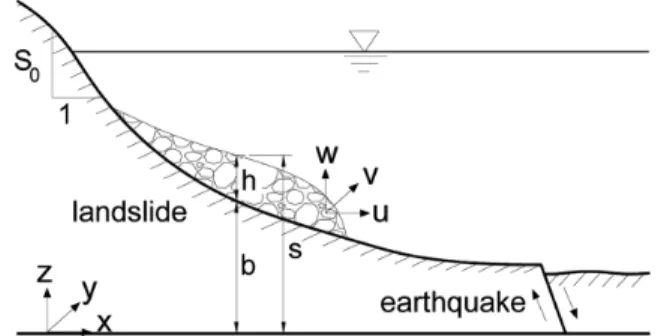
Fig. 1 shows the computational domain for simulating submarine landslide and defined variables. In the figure, s and b are the elevations of the surface and bottom of the debris from a reference line, h (= s− b) is the debris depth,

and (u, v, w) are the velocities in the (x, y, z) directions. The continuity equation for the incompressible fluid flow is given by

(1)

Boundary conditions at the surface and bottom of the debris are as follows:

(2)

(3)

We integrate Eq. (1) from the bottom to the surface and use the Leibnitz’s rule with the boundary conditions given by Eqs. (2) and (3). Finally, we get the continuity equation in two-dimensional (x, y) domain as

(4)

and the continuity equation in one-dimensional (x) domain as

(5)

The x-directional momentum equation is defined as follows:

(6)

where τxx, τyx, τzx are the shear stresses. We only consider the x − z plain, so τxx, τyx are equal zero. In Eq. (6), the pressure p is assumed to be hydrostatic and thus p = ρg(s − z). We add u(∂u/∂x + ∂v/∂y + ∂w/∂z) to Eq. (6) in order to get the

∂u∂x --- + ∂v

∂y--- + ∂w --- = 0∂z

∂s∂t --- + u∂s

∂x--- + v∂s

∂y--- − w = 0, z = s

∂b --- + u∂∂t b

∂x--- + v∂b

---∂y − w = 0, z = b

∂t∂

---- s − b( ) + ∂∂x--- s − b[( )u] + ∂∂y--- s − b[( )v] = 0

∂t∂

---- s − b( ) + ∂∂x--- s − b[( )u] = 0

∂u --- + u∂∂t u

∂x--- + v∂u --- + w∂∂y u

---∂z

= − 1 ρ---∂p

∂x--- + 1 ρ--- ∂τxx

--- + ∂x ∂τyx

--- + ∂y ∂τzx

---∂z

⎝ ⎠

⎛ ⎞

Fig. 1. Computational domain of submarine landslide using the coordinate of (b, s).

(3)

following equation

(7)

where − ∂b/∂x(= S₀) is the bottom slope. We integrate Eq.

(7) from the bottom to the surface, use the Leibnitz’s rule and the boundary conditions given by Eqs. (2) and (3).

After neglecting the shear stress at the free surface, the resulting momentum equation is given as

(8)

In one-dimensional (x) domain, Eq. (8) is reduced to

(9)

which can also be expressed as

(10) using the following relation as τzx

z=b=ρg(s − b)Sf. Follow- ing Voellmy (1955) type of the flow resistance relation, the friction term S_f may consist of two components, i.e., the bottom friction and the internal soil friction given by

(11) where n and μ are the Manning’s roughness and the effective friction coefficients, respectively. Manning’s n values range from 0.032 to 0.2 s/m^1/3 while the μ values for debris flows range from 0.06 to 0.175 (Paik, 2015).

Eqs. (5) and (10) are the one-dimensional shallow water equations in a conservative form to deal with numerical discontinuities in landslides. Using chain rule and the continuity Eq. (5), the momentum Eq. (10) becomes

(12)

and, further dividing by (s− b), the resulting momentum equation is given by

(13)

Eqs. (5) and (13) are the one-dimensional shallow water equations in an alternative conservation form (Toro, 2001).

2.2 Numerical scheme

In the present model, a finite volume scheme with an approximate Riemann solver is used to discretize the governing equations in time. The governing equations of the one-dimensional shallow water equations can be written in a conservative form as

(14)

where

(15)

(16)

(17)

and U is the vector of conserved variables. Eq. (14) is solved using the splitting method. At the first step, the homogenous pure advection problems are solved as

(18)

(19) where the superscript “n” implies the present time step and the subscript “i” implies the cell center of the computational domain. At the second step, the final solutions of U are obtained by adding the source terms as

(20)

(21) where U_i^(s) is the value at which the source term vector S is evaluated. To avoid numerical instability due to the friction term, an implicit scheme is employed following Paik (2015).

The WAF (weighted average flux) method is known as the second-order extension of the Godunov method. A TVD (total variation diminishing) version of the WAF method

∂u --- + ∂∂t u²

--- + ∂∂x uv --- + ∂∂y uw

--- + g∂∂z (s − b) ---∂x

= − g∂b

∂x--- + 1 ρ---∂τzx

---∂z

∂ s − b[( )u]

--- + ∂∂t [(s − b)u²]

--- + ∂∂x [(s − b)uv] ---∂y + 1

2---g∂[(s − b)²]

--- = g s − b∂x ( )S₀ − 1 ρ---τzx

z=b

∂ s − b[( )u]

--- + ∂∂t [(s − b)u²] --- + ∂x 1

2---g∂[(s − b)²] ---∂x

= g s − b( )S₀ − 1 ρ---τzx

z=b

∂ s − b[( )u]

--- + ∂∂t [(s − b)u²] --- + ∂x 1

2---g∂[(s − b)²] ---∂x

= g s − b( ) S( ₀ − Sf)

S_f = n²u u s − b ( )^4/3

--- + μcosθ

s − b ( ) ∂u

--- + u∂∂t u

∂x--- + g∂(s − b) ---∂x

= g s − b( ) S( ₀ − Sf)

∂u --- + ∂∂t

∂x--- 1 2---u² + gs

⎝ ⎠

⎛ ⎞ = − n²u u s − b ( )^4/3

--- − μcosθ

∂U

--- + ∂∂t F U( ) --- = H U∂x ( )

U = s − b s − b

( )u

⎝ ⎠

⎜ ⎟

⎛ ⎞

F U( ) = (s − b)u s − b

( )u² + 1

2---g s( − b)²

⎝ ⎠

⎜ ⎟

⎛ ⎞

H U( ) = g s − b( ) S₀ − n²u u s − b ( )^4/3

--- − μcosθ

∂U∂t

--- + ∂F U( ) --- = 0∂x

U_i⁽^adv⁾ = U_iⁿ − Δt

Δx--- F[ _i+1/2 − Fi−1/2]

dU --- = H Udt ( )

U_iⁿ⁺¹ = U_i^adv + ΔtS U( _i^{( )}^s)

(4)

which results in a high-resolution method is employed in this study. Thus, the numerical flux at the cell interface can be expressed as

(22)

where c_k(= S_kΔt/Δx) is the Courant number related to the wave speed S_k. The flux jump across wave k at the cell interface is given by

(23) and the WAF limiter function is given by

(24) where

(25) and r^(k) is the ratio of the upwind change to the local change.

B(r^(k)) is the limiter function (Toro, 2001). In this study, we use the van Leer limiter function for B(r) as

(26)

The HLL approximate Riemann solver is used to determine the HLL numerical flux as

(27)

The wave speed estimates are given as

(28)

In Eq. (28), where K = L, R is the wave celerity and q_K is given by

(29)

where

(30) For wet/dry bed conditions, the wave speeds are deter- mined as

(31)

(32)

2.3 CFL criterion

The numerical scheme used in this study is explicit and the CFL (Courant-Friedrichs-Lewy) number is investigated for numerical stability. The speed of landslides, especially for the wet/dry front speed, can be affected by the friction slope terms. In this study, we use a new CFL criterion (Paik, 2015) to determine the time step given by

(33)

where c is the celerity, u_f is the total friction velocity. In the Voellmy resistance relation, the total friction velocity can be expressed as

(34)

The value of 0.9 of the CFL number is used for all the simulations in this study.

3. Model Validation for Water Flow and Debris Flow

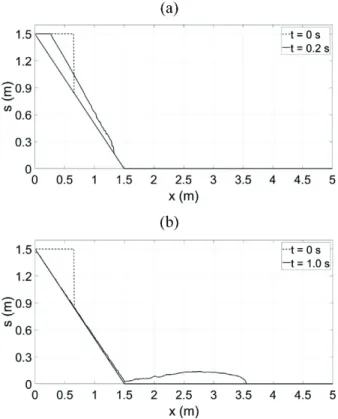
3.1 Validation for water flow after dam break In the first part, we validate conservative forms of the equations for a dam-break problem. We compare solutions of conservative forms of the governing Eqs. (5) and (10) and alternative conservative forms of the governing Eqs. (5) and (13) using homogeneous parts of these equations. The computational domain is 2 m long, a dam is located in the middle of the domain and water of 0.1 m depth is located behind the dam. Figs. 2(a) and 2(b) show numerical solutions of water surface elevations at t = 0.2 s using the conservative forms and alternative conservative forms, respectively. In the figures, analytical solutions (Mangeney et al., 2000) as well as initial conditions are shown for comparison. The conservative forms of the equations yield the same solutions as the analytical solutions. However, the alternative conservative forms of the equations yield different solutions. At a point of dry bed, (s− b) is equal to zero. In deriving alternative conservative forms of the momentum Eq. (13), we divide some terms by zero-valued (s− b) F_i+1/2 = 1

2--- F( _i + F_i+1) − 1

2--- sign c( )A_k i+1/2 k ΔFi+1/2

k k=1

∑

2

ΔFi+1/2

k = F_i+1/2^k+1 − Fi+1/2 k

A_i+1/2^k = A_i+1/2^k (r^{( )}^k, c_k)

A r( ) = 1 − 1 − c^{( )}^k ( k)B r( )^{( )}^k

B r( ) = 2r 1 + r ---

F_i+1/2^HLL

=

F_L, if 0 S≤ _L

S_RF_L − SLF_R + S_RF_L(U_R − UL) S_R − SL

---, if S_L≤ ≤0 S_R

F_R, if S_R≤0

⎩⎪

⎪⎨

⎪⎪

⎧

S_L = u_L − aLq_L S_R = u_R − aRq_R

a_K = g s( K − bK)

q_K = 1

2--- (h_* + h_K)h_* h_K²

--- , if h_*>h_K 1, if h_*≤h_K

⎩⎪

⎨⎪

⎧

h_* = a[( _L + a_R)/2 + u( L − uR)/4]²/g

S_L = u_R − 2aR, if (h_L = 0, h_R>0) u_L − aL, if (h_L>0, h_R = 0)

⎩⎨

⎧

S_R = u_L + 2a_L, if (h_L>0, h_R = 0) u_R + a_R, if (h_L = 0, h_R>0)

⎩⎨

⎧

Δt = CFL Δx

max u , u( _f) + c ---

u_f = g s − b( ) n²u² s − b ( )^4/3

--- + μcosθ

⎝ ⎠

⎛ ⎞ ^1/2

(5)

which is mathematically meaningless. That is why numerical solutions of alternative form of the equations are different from the analytical solution in the dry/wet discontinuity points. In further investigation, we use the conservative forms of the equations only.

In the second part, we compare our model results with two cases with physical experimental data for water flow after dam break. The first case was done by Stansby et al.

(1998). The test conditions are the same as in the first part.

That is, the domain is 2 m long, a dam is located in the middle, and water with 0.1 m depth is located behind the dam.

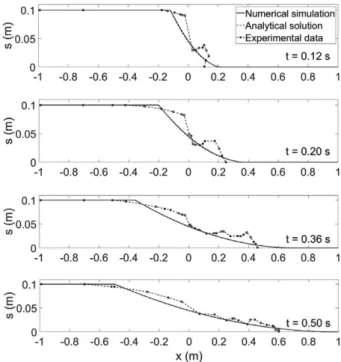
Fig. 3 compares numerical solutions, analytical solutions, and the measured data at t = 0.12 s, 0.20 s, 0.36 s, 0.50 s.

On the whole, the numerical results show good agreements with the analytical solutions and the experimental data even though wave breaking occurred in reality. Especially, the numerical solutions are closer to the measured data at t = 0.36 s and t = 0.50 s when the water surface elevations are milder than at previous times.

The second case was done by Liang and Marche (2009) who tested a large-scale dam-break flow over a symmetric triangular hump as shown in Fig. 4. The domain is 38m long and a dam is located 15.5 m away from the upstream end. Water of 0.75 m depth fills the dam. The triangular hump is 0.6 m long and 0.3 m high and the center of it is located 13 m away from the dam. To investigate sensitivity

of the flow on the bottom friction, three Manning’s roughness coefficients are set as n = 0.00833 m^−1/3s, 0.0125m^−1/3s, 0.01875 m^−1/3s which are different with a ratio of 1.5 each other. The upstream boundary is closed while the downstream boundary is open. Liang and Marche (2009) measured time series of water depths at 7 gauges which are located at 2 m, 4 m, 8 m, 10 m, 11 m, 13 m, and 20 m downstream of the dam. For numerical experiment, the total simulation time is 90 s and the grid size is 5 cm.

Time series of water depths at 7 gauges are recorded to describe these complicated phenomena and compared with the experimental data in Fig. 5. At the initial time, the dam suddenly broke and the initial water at the reservoir rushed onto the downstream like a flood on a plain. The waterfront reached the left slope, climbed over the peak of the hump (gauge 1 to 6) and further arrived at the other side of the Fig. 2. Comparison of numerical solutions of water surface eleva-

tions against analytical solutions at t = 0.2 s after dam break:

(a) conservative form; (b) alternative conservative form.

Fig. 3. Comparison of numerical solutions, analytical solutions and experimental data of water surface elevations at different time steps after dam break.

Fig. 4. Computational domain for dam break flow over a triangular hump.

(6)

horizontal bottom (gauge 7) around t = 5 s. Because of an interaction between the incoming waves and the reflecting waves from the side of the hump, a shock wave formed and propagated back to the upstream boundary. On the other side of the hump, a rarefaction wave occurred and moved to the downstream boundary, which caused increase of water depth at the right side of the hump (gauge 7). Around t = 25 s, the shock wave reached and reflected from the wall at the upstream boundary. After this reflection, the second wave propagated to the downstream. These complex processes continued until the momentum energy was damped due to bottom friction and water mass passed through the downstream boundary.

Overall, the numerical simulations show good agreements with the experimental data in term of both the propa-

gation speed and water depth. In particular, at gauges 1 and 2, numerical results are close to the measured data until t = 90 s. At gauges 3 to 6, numerical results around the first peak of water depths are higher than the measured data. At gauge 7 which is at the other side of the hump, numerical results are always higher than the measured data. These dis- crepancies might happen because the numerical solutions of the shallow water equations were made based on the assumption of neglecting dispersive terms which would spread out several components with different speeds. If we simulate these flow phenomena using the Boussinesq equations which include dispersive terms, we would get solutions closer to the experimental data. When the Manning’s roughness coefficient n increases, the flow speed decreases at the first wave and the flow thickness increases at all the 7 Fig. 5. Comparison of numerical results of water depth with experimental data at 7 gauges for dam-break flow over a hump.

(7)

gauges. Especially, at gauges 3 to 6, due to the adverse slope of the hump, with the increase of the Manning’s n, the flow thickness decreases at the first peak. The Manning’s n equal to 0.0125 gives the numerical solutions closest to the measured data.

3.2 Validation for debris flow

The present landslide model is applied for debris flow on the well-known large-scale USGS experimental flume. This experiment which was conducted on September 13, 2001 (Iverson, 2003; Iverson et al., 2010) has been investigated by several researchers to test their debris flow models (Den- linger and Iverson, 2001; Paik, 2015). The flume is a rect- angular concrete channel, 95 m long, 2 m wide, and 1.2 m deep. The main part of the channel has a steep slope of 31^o and is connected with a curve to the runout surface having a mild slope of 2.4^o. The debris flow from the main channel would deposit at the 4 m wide runout surface. A volume of saturated soil has a mass of 9.4 m³ consisting of sand-gravel- mud (SGM) material and is suddenly opened by a vertical headgate. More detailed information about the experimental facilities was reported in Iverson (2003) and Iverson et al. (2010).

Numerical simulation is conducted using the soil den- sity of ρ = 2100 kg/m³, the Manning’s roughness coefficient of n = 0.034 m^−1/3s, and the effective friction coefficient of μ = 0.12. The grid size is 0.1 m and the CFL number is 0.9 which guarantees numerical stability. During simulation we use a constant value of 2 m channel width because the numerical model is horizontally one dimensional. In the real experiment, however, the width changed from 2 m at the main channel to 4 m at the runout surface.

This width change would cause numerical solutions different from the experimental data on the area of the runout surface.

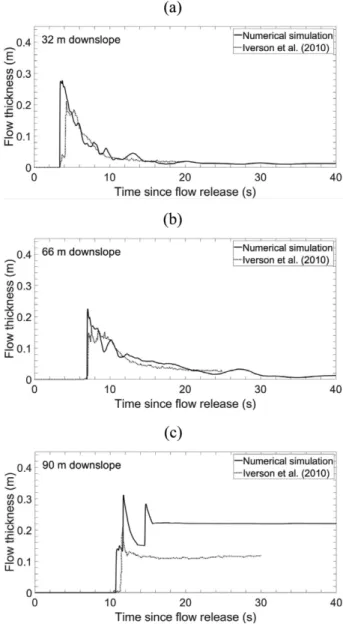
Fig. 6 compares numerical results of debris flow thickness with measurement data at locations of x = 32 m, 66 m, 90 m downstream of the headgate. It should be noticed that the location x is not the horizontal distance but the downslope distance on the bottom. The first and second locations are in the main channel while the third location is on the runout surface. Due to turbulent high speed of the debris flow on the steep channel, high fluctuation of the solutions occurred at the first and second locations in the present high-resolution numerical model. To smooth the highly fluctuating solutions, we use the moving average algorithm as given by

(35)

where y_k is the raw (noisy) data, (y_k)_s is the smoothed data, the odd number 2n + 1 is named as the filter width or span.

The greater the filter width is, the smoother the data are. In order to smooth these time series data of the flow thickness, we choose the value of span 2n + 1 = 101 which is equiva- lent to value of n = 50 and repeat smoothing process again.

The results after smoothing are shown in Figs. 6(a) and 6(b).

On the whole, the numerical simulations are in good agreement with the experimental data, especially in term of the flow speed and flow thickness. Although the ampli- tudes are overestimated, the peakedness and the fluctuation of the computed results represent the effects of friction terms in the momentum equation. The peaks of the simulat-

y_k

( )_s = y_k+i 2n + 1 ---

i=−n i=n

∑

Fig. 6. Comparison of numerical results of debris flow thickness with experimental data, (a) 32 m downslope, (b) 66 m downslope, (c) 90 m downslope.

(8)

ing results are higher than the measurement data due to the assumption of being hydrostatic in the shallow water equations as mentioned in the previous test. The time series data which are measured at x = 32 m and x = 66 m in Fig. 6(a) and Fig. 6(b), respectively, show better agreements than those at x = 90 m. These differences are of the curvature connected between bed slope of 31^o and the flat bottom of 2.4^o is not represented well in this simulation. Moreover, in the present 1D model, the width of the channel of 2 m is taken into account for the whole domain while that of runout surface of 4 m is set at this point of the experiment as mentioned previously. It results in the overestimation of approximate 50% in term of the flow thickness on the runout surface.

4. Model Application to Subaerial and Submarine Landslides

The debris flows over and under the water surface are called as the subaerial and submarine landslides, respectively. The subaerial landslide is affected by the subaerial gravity acceleration g₀= 9.81 m/s² whereas the submarine landslide is affected by the buoyancy gravity acceleration g₁= g₀(ρs− ρw/ρs where ρs andρw are densities of soil and water, respectively. Rzadkiewicz et al. (1997) conducted hydraulic experiment of a submarine landslide and the induced tsunami. The volume of soil in a triangular section with 0.65 m × 0.65 m suddenly slid down on a slope of 45^o which was connected to a horizontal bottom and the tsunami occurs due to the landslide. They also simulated the phenomenon using 2-dimensional (x, z) Navier-Stokes equations. In this study, we conduct numerical experiments of subaerial and submarine landslides using their model scales (see Fig. 7).

Fig. 7. Topography of subaerial and submarine landslides on a slope of θ = 45^o connected to a horizontal bottom.

Fig. 8. Numerical result of soil surface elevations at t = 0.4 s for subaerial landslide.

Fig. 9. Numerical result of soil surface elevations at t = 0.4 s for submarine landslide.

Fig. 10. Numerical result of soil surface elevations at t = 0.4 s for combined subaerial-submarine landslide.

However, we use different properties of ρ = 2100 kg/m³, n = 0.034 m^−1/3s, μ = 0.08 following Paik (2015) who simulated landslides using the Saint-Venant equations. The grid size is Δx = 1 cm and the CFL number is 0.9 which guarantees a numerical stability.

Figs. 8 and 9 show surface elevations of the subaerial and submarine landslides, respectively, at t = 0.4 s. For the submarine landslide, due to the buoyancy effect, the acceleration is reduced to g₁= 0.52g₀ and the soils move more slowly compared to the subaerial landslide.

Fig. 10 shows surface elevations of combined subaerial- submarine landslide at t = 0.4 s for the water surface at s_w=

(9)

0.8 m. Subaerial landslide occurs above the water surface while submarine landslide occurs below the water surface.

For the submarine landslide, due to the buoyancy effect, the acceleration is reduced to g₁= 0.52g₀ and the soils move more slowly compared to the subaerial landslide. There- fore, for this combined subaerial-submarine landslide, the soils move more slowly compared to the subaerial landslide (Fig. 8). However, they move faster compared to the submarine landslide (Fig. 9).

The next case study is to investigate the sensitivity of debris flow with different parameters. We change the angle of slopes from θ = 45ô to θ = 30ô. Fig. 11 shows the topography for simulating subaerial landslide with bottom slope of θ = 30ô.

Fig. 12 shows the numerical solutions of surface elevations of subaerial landslide with bottom slope of θ = 30^o at t = 0.4 s. After comparison with the solution with θ = 45^o shown in Fig. 8, we find that the velocity increases with the increase of the bottom slope. These results are physically reasonable.

Furthermore, we compare numerical results with different Manning’s roughness coefficient of n = 0.034 m^−1/3s and n = 0.051 m^−1/3s which are different with a ratio of 1.5. It is clear that the propagation speed of the debris flow depends on the bottom roughness coefficient.

Figs. 13 and 14 show numerical solutions of surface elevations of subaerial landslide with Manning’s n of 0.034 m^−1/3s and 0.051 m^−1/3s, respectively. The speeds of landslides of Fig. 11. Topography for simulating subaerial landslide with bot-

tom slope of θ = 30^o.

Fig. 12. Numerical result of soil surface elevations at t = 0.4 s for subaerial landslide with bottom slope of θ = 30^o.

Fig. 13. Numerical result of soil surface elevations for subaerial landslide with n = 0.034 m^−1/3s, (a) t = 0.2 s, (b) t = 1.0 s.

Fig. 14. Numerical result of soil surface elevations for subaerial landslide with n = 0.051 m^−1/3s, (a) t = 0.2 s, (b) t = 1.0 s.

(10)

the two cases are slightly different at t = 0.2 s, but the two speeds become more clearly different at t = 1.0 s. This implies that larger bottom roughness cause slower speed of the debris flow which was mentioned also by the previous works (Mikoš et al., 2006; Paik, 2015).

5. Conclusions

In this study, we investigated subaerial and submarine landslides using the finite volume scheme in the one-dimensional (x) shallow water equations. We used the (b, s) coordinate system to express the shallow water equations which can be applied in coastal zone as well as river. To discretize the governing equations, we used the well-known high-resolution scheme which combines the TVD limiter function and the second-order Godunov method (WAF method) employing HLL approximate Riemann solver. This scheme can deal with the wet/dry problems occurring in the real landslide phenomena. We applied both the conservative and alternative conservative forms of the shallow water equations to a dam-break water flow and found that the conservative form of the equations yielded accurate solutions in the dry/wet boundaries but the alternative conservative form yielded inaccurate solutions. We further verified the developed numerical model by comparing numerical results with the analytical solutions and the experimental measurements for both the dam-break water flow and the debris flow. We also applied the model to subaerial landslides with different bottom slopes and bottom frictions and found that both steeper bottom slope and smaller bottom friction cause faster movement of soils. In the future, the two-dimensional (x, y) shallow water equations as well as the non-hydrostatic equations (e.g., the Boussinesq equations) will be developed to accurately solve the subaerial and submarine landslide phenomena.

Acknowledgements

This research was supported by Technology Advance- ment Research Program (TARP) funded by the Ministry of Land, Infrastructure and Transport of Korean government (No. 19CTAP-C152942-01).

References

Denlinger, R.P. and Iverson, R.M. (2001). Flow of variably fluid- ized granular masses across three-dimensional terrain: 2.

Numerical predictions and experimental tests. Journal of Geo- physical Research: Solid Earth, 106, 553-566. https://doi.org/

10.1029/2000JB900330.

Erduran, K.S., Kutija, V. and Hewett, C.J.M. (2002). Performance of finite volume solutions to the shallow water equations with shock-capturing schemes. International Journal for Numerical Methods in Fluids, 40, 1237-1273. https://doi.org/10.1002/

fld.402.

Horrillo, J., Wood, A., Kim, G.-B. and Parambath, A. (2013). A simplified 3-D Navier-Stokes numerical model for landslide- tsunami: Application to the Gulf of Mexico: A Simplified 3-D Tsunami Numerical Model. Journal of Geophysical Research:

Oceans, 118, 6934-6950. https://doi.org/10.1002/2012JC008689.

Imran, J., Parker, G., Locat, J. and Lee, H. (2001). 1D Numerical Model of Muddy Subaqueous and Subaerial Debris Flows.

Journal of Hydraulic Engineering, 127, 959-968. https://doi.org/

10.1061/(ASCE)0733-9429(2001)127:11(959).

Iverson, R.M. (2003). The debris-flow rheology myth. Debris Flow Mechanics and Mitigation Conference. Mill Press, Davos, 303- 314.

Iverson, R.M. (2015). Scaling and design of landslide and debris- flow experiments. Geomorphology, 244, 9-20. https://doi.org/

10.1016/j.geomorph.2015.02.033.

Iverson, R.M., Logan, M., LaHusen, R.G. and Berti, M. (2010).

The perfect debris flow? Aggregated results from 28 large-scale experiments. Journal of Geophysical Research, 115, F03005.

https://doi.org/10.1029/2009JF001514.

Jakob, M., Anderson, D., Fuller, T., Hungr, O. and Ayotte, D.

(2000). An unusually large debris flow at Hummingbird Creek, Mara Lake, British Columbia. Canadian Geotechnical Journal, 37, 1109-1125.

Liang, Q. and Marche, F. (2009). Numerical resolution of well-bal- anced shallow water equations with complex source terms.

Advances in Water Resources, 32, 873-884. https://doi.org/

10.1016/j.advwatres.2009.02.010.

Major, J.J. (1997). Depositional Processes in Large-Scale Debris- Flow Experiments. The Journal of Geology, 105, 345-366.

https://doi.org/10.1086/515930.

Mangeney, A., Heinrich, P. and Roche, R. (2000). Analytical Solu- tion for Testing Debris Avalanche Numerical Models. Pure and Applied Geophysics, 157, 1081-1096. https://doi.org/10.1007/

s000240050018.

McDougall, S., Boultbee, N., Hungr, O., Stead, D. and Schwab, J.W. (2006). The Zymoetz River landslide, British Columbia, Canada: description and dynamic analysis of a rock slide-debris flow. Landslides, 3, 195-204. https://doi.org/10.1007/s10346- 006-0042-3.

Mikoš, M., Fazarinc, R., Majes, B., Rajar, R., Žagar, D., Krzyk, M., Hojnik, T. and Četina, M. (2006). Numerical simulation of debris flows triggered from the Strug rock fall source area, W Slovenia. Natural Hazards and Earth System Science, 6, 261- 270. https://doi.org/10.5194/nhess-6-261-2006.

Naef, D., Rickenmann, D., Rutschmann, P. and McArdell, B.W.

(11)

(2006). Comparison of flow resistance relations for debris flows using a one-dimensional finite element simulation model. Nat- ural Hazards and Earth System Science, 6, 155-165. https://

doi.org/10.5194/nhess-6-155-2006.

Paik, J. (2015). A high resolution finite volume model for 1D debris flow. Journal of Hydro-environment Research, 9, 145- 155. https://doi.org/10.1016/j.jher.2014.03.001.

Rzadkiewicz, S.A., Mariotti, C. and Heinrich, P. (1997). Numerical Simulation of Submarine Landslides and Their Hydraulic Effects. Journal of Waterway, Port, Coastal, and Ocean Engi- neering, 123, 149-157. https://doi.org/10.1061/(ASCE)0733- 950X(1997)123:4(149).

Sassa, K., Dang, K., Yanagisawa, H. and He, B. (2016). A new landslide-induced tsunami simulation model and its application to the 1792 Unzen-Mayuyama landslide-and-tsunami disaster.

Landslides, 13, 1405-1419. https://doi.org/10.1007/s10346-016- 0691-9.

Stansby, P.K., Chegini, A. and Barnes, T.C.D. (1998). The initial stages of dam-break flow 18.

Tappin, D.R., Grilli, S.T., Harris, J.C., Geller, R.J., Masterlark, T., Kirby, J.T., Shi, F., Ma, G., Thingbaijam, K.K.S. and Mai, P.M.

(2014). Did a submarine landslide contribute to the 2011 Tohoku

tsunami? Marine Geology, 357, 344-361. https://doi.org/10.1016/

j.margeo.2014.09.043.

Toro, E.F. (2001). Shock-capturing methods for free-surface shallow flows. John Wiley & Sons, LTD.

Van Tien, P., Sassa, K., Takara, K., Fukuoka, H., Dang, K., Shiba- saki, T., Ha, N.D., Setiawan, H. and Loi, D.H. (2018). Forma- tion process of two massive dams following rainfall-induced deep-seated rapid landslide failures in the Kii Peninsula of Japan.

Landslides, 15, 1761-1778. https://doi.org/10.1007/s10346-018- 0988-y.

Voellmy, A. (1955). Uber die Zertorungskraft von Lawinen. Sch- weizerische Bauzeitung. Schweizerische Bauzeitung, 73, 212- 285.

Yavari-Ramshe, S., Ataie-Ashtiani, B. and Sanders, B.F. (2015). A robust finite volume model to simulate granular flows. Com- puters and Geotechnics, 66, 96-112. https://doi.org/10.1016/

j.compgeo.2015.01.015.

Received 19 August, 2019 Accepted 26 August, 2019