Geosciences Journal
Vol. 11, No. 4, p. 357 − 367, December 2007
Sulfur and oxygen isotopic compositions of the dissolved sulphate in the meteoric water in Chuncheon, Korea
ABSTRACT: The meteoric water deposited in the Chuncheon area was collected from July 2002 to May 2004 and its chemical and isotopic compositions were analyzed to examine if the isotopic data can help trace the sources of the sulfur pollutant and under- stand the details of acid formation processes in the air. The chem- ical compositions of the meteoric water indicate that the sulfate mostly comes from anthropogenic sources. The sulfur isotopic compositions of the dissolved sulfate in the meteoric water ( δ
34S
SO4) vary from 2.6 to 7.5‰ with little seasonal differences, which are significantly different from those of the sulfur in the coal being locally consumed ( −4.5 to −0.7‰). This difference indicates that the local coal consumption gives insignificant contribution to the pollutant sulfur in the acid deposition of the area. The relationship between δ
34S
SO4and the concentration of sulfate suggests that the sources of pollutant sulfur are variable and inhomogeneous. The oxygen isotopic compositions of the dissolved sulfate in the mete- oric water ( δ
18O
SO4) range from 9.0 to 17.2‰, which are generally lower in winter than in spring. Comparison between the measured and calculated values of δ
18O
SO4suggests that the oxygen isotopic exchange between sulfite and water occurs before its oxidation to sulfate. The extent of isotopic exchange seems to be not controlled by equilibrium but by kinetic fractionation. The poor correlation between δ
18O
SO4and the oxygen isotopic composition of the meteoric water confirms the disequilibrium nature of the isotopic exchange.
Key words: sulfur and oxygen isotope, meteoric water, pollutant sulfur sources, acid forming processes
1. INTRODUCTION
The rapid industrial growth of East Asia forces the coun- tries in the region, including Korea, Japan, and China, to face a number of serious environmental problems. One of the environmental problems more concerned is the acid deposition caused by the anthropogenic sulfur and nitrogen emission into the air. Sulfur has been considered to be a greater contributor to the acid deposition than nitrogen, although the importance of nitrogen is increasing as the controls on sulfur emission have been tightened in recent years (Han et al., 2006). The chemical compositions of the
precipitation from Yu and Park (2004) and Jeon and Chung (2005) indicated that pollutant sulfur plays bigger role in forming acid deposition than nitrogen in the southern Korean peninsular.
Like most of the other air pollutants, sulfur can travel a fairly long distance and make a transboundary pollution.
Since there has been dispute on the estimation on the amount of transboundary pollution of sulfur, especially in East Asia (Huang et al., 1995; Ichikawa and Fujita, 1995;
Streets et al., 2000; Carmichael et al., 2002), the sulfur pol- lution may raise a delicate conflict among neighboring countries in the region. An appropriate estimation of the transboundary pollution may first require tracing the sources of the acid and understanding the principles of the acid formation. Tracing the sources of the pollutant sulfur has mostly relied on the physical models (e.g. Dastoor and Pudykiewicz, 1996). An addition of another tracer, e.g. a chemical or an isotopic tracer, to the physical models can enhance the efficiency and accuracy of the source tracking.
Isotopic compositions of the acids in the precipitation can be used as an effective tool for tracing the acid sources and elucidate the details of the acid formation processes. The sulfur isotopic compositions ( δ
34S) of atmospheric sulfur dioxide (SO
2) or sulfate (SO
4) have been investigated to trace the sulfur sources, as summarized by Krouse (1980) for the researches before 1980. Recently, Na et al. (1995), Ohizumi et al. (1997), McArdle et al. (1998) Pichlmayer et al. (1998), Panettiere et al. (2000), and Yu and Park (2004) studied δ
34S of sulfate ( δ
34S
SO4) in the atmospheric precip- itation. The results from these previous investigations show that the δ
34S values of atmospheric pollutant sulfur are gen- erally lower than that of sea sulfate and could be indicative of the pollution sources. In many cases, however, the sources not only produce variable amount of sulfur but also have inhomogeneous δ
34S values (Krouse, 1980), which may be partly responsible for the disagreements in identifying the sources of sulfur pollutants among investigations.
Sulfur is mainly emitted as SO
2, most of which is prob- ably an oxidation product of sulfide in the fossil fuels dur- ing combustion. SO
2is hydrated to sulfite (SO
3) and then Jae-Young Yu*
Youngyun Park
†Randall E. Mielke Max L. Coleman
} }
Department of Geology, Kangwon National University, Chuncheon, Kangwon-Do 200-701, Korea Center for Life Detection, Jet Propulsion Laboratory, 4800 Oak Grove Drive, Pasadena, CA 91109, USA
*Corresponding author: [email protected]
†
Present address: Environmental Tracer Team, Korea Basic Science
Institute, 52 Yeon-dong, Yusung-gu, Daejeon 305-333, Korea
further oxidized to SO
4which forms sulfuric acid causing acid rain:
M-S + 3O
2→ MO + SO
2, (R1)
SO
2+ H
2O → H
2SO
3, and
39)(R2)
H
2SO
3+ 0.5O
2→ H
2SO
4(R3)
As shown in the above reactions, the oxygen in the sulfur oxides comes from two sources; water and free oxygen whose isotopic compositions are remarkably different. The oxygen isotopic composition of meteoric water ( δ
18O
w) is commonly less than 0‰ (Epstein and Mayeda, 1953; Tor- ran and Harris, 1989), while that of free oxygen ( δ
18O
a) is 23.5‰ (Kroopnick and Craig. 1972). This big difference in δ
18O between the two sources may enable to estimate the relative contribution of each source to the sulfate oxygen with the oxygen isotopic composition of sulfate ( δ
18O
SO4) and to check if the estimated contribution is pertinent to that expected from the stoichiometry given by the above reac- tions. The investigations on δ
18O
SO4, however, have been relatively rare. A few studies on δ
18O
SO4showed that the oxygen in sulfate mainly originates from water (Lloyd, 1968; Mizutani and Rafter, 1969; Cortecci and Longinelli, 1970; Holt et al., 1981), which is quite contrary to what the stoichiometry of the above reactions suggest, that is, most of the sulfate oxygen should come from free oxygen.
The purposes of this study are to examine δ
34S
SO4and δ
18O
SO4in the meteoric water in Chuncheon, Korea, and to see if the combination of these two isotopes helps trace the sources of the sulfur pollutant and understand the acid for- mation processes further. As mentioned earlier, δ
18O
SO4is rarely investigated and this study is probably one of the few combining sulfur and oxygen isotopes for the investigation on pollutant sulfur.
2. METHODS
Samples of meteoric water (rain + snow) were collected at each precipitation event with a homemade sampler placed at the top of Natural Science building 3 of Kangwon National University in Chuncheon from July 2002 to May 2004. The collected water samples were filtered through a 0.2 μm micropore membrane and an aliquot of 250 ml of each filtered sample was acidified with approximately 0.2 ml HNO
3. The filtered and acidified samples were refrigerated at 4
oC for later analysis. The samples of the coal and petro- leum being locally consumed for heating and automobiles were also collected.
The pH, Eh, conductivity (K
25) and temperature (T) of water samples were measured when the samples were being collected at the site. The alkalinities of the water samples were determined using Gran method (Wetzel and Likens, 1991) on a 50 ml aliquot of the filtered sample on the same day of sample collection. The carbonate concentrations were calculated from the measured alkalinities assuming that
only carbonates significantly contribute to the alkalinity (Stumm and Morgan, 1981). The chemical compositions of the water samples were analyzed with an inductively cou- pled plasma atomic emission spectrometer (ICP-AES; for Si, Al, Ca, Mg, K, and Na) at the Seoul Branch of the Korean Basic Science Institute (KBSI) and an ion chro- matograph (IC; for NH
4, Cl, NO
3, and SO
4) at the Depart- ment of Geology, Kangwon National University.
δ
18O
wand hydrogen isotopic compositions of water ( δD
w) were obtained from the analysis of CO
2equilibrated with the water (Epstein and Mayeda, 1953) and H
2released from the water by Zn-reduction (Coleman et al., 1982), respectively.
The dissolved sulfate in the water samples was precipitated as BaSO
4(Kolthoff et al., 1969), which was then analyzed for sulfur and oxygen isotopic compositions. δ
34S
SO4was determined by analyzing SO
2released from the BaSO
4mixed with V
2O
5and quartz glass at 1120
oC (Yanagisawa and Sakai, 1983). δ
18O
SO4was measured with CO generated from the mixtures of BaSO
4and Ag
2S in the presence of graphite and glassy carbon in the Finnigan Thermal Com- bustion/Elemental Analyzer (TC/EA) at 1450
oC. Sulfur in the petroleum samples were attempted to extract with com- bustion in an oxygen bomb (Na et al., 1995) and in a fur- nace while the exhaustion gas was being bubbled through 1% H
2O
2solution (Lodge, 1990). None of these methods gave enough sulfur for isotopic analyses of petroleum. Sul- fur in the coal samples were extracted by igniting coal with CuO in an electric furnace, from which the evolved SO
2was directly trapped and analyzed.
The standards for reporting the isotopic compositions are Standard Mean Oceanic Water (SMOW) for δ
18O and δD and the troilite from Cañon Diablo meteorite (CDT) for δ
34S. All the isotopic analyses except δ
18O
SO4were per- formed with a mass spectrometer, model PRISM II of Micromass UK Ltd. at KBSI in Daejeon, Korea. δ
18O
SO4were measured with Finnigan Conflo III and Finnigan MAT 253 SIR-MS in Jet Propulsion Laboratory (JPL) in Pasa- dena, USA. The reference materials used in the analyses were: SMOW ( δ D=0.0‰) and SLAP (δ D=428‰) from International Atomic Enery Agency (IAEA) for δD
w; KBSI Lab standard KBSI-27 ( δ
18O=9.6‰) and SMOW (δ
18O=0.0‰) for δ
18O
w, NBS-127 BaSO
4( δ
34S=20.3‰) for δ
34S
SO4, NBS- 127 BaSO
4( δ
18O=8.6‰) and JPL Lab standard BaSO
4( δ
18O=11.6‰) for δ
18O
SO4, and NBS-123 sphalerite ( δ
34S=
17.4‰) for δ
34S of coal. The standard errors of the mea- surements were estimated to be less than 2‰ for δD
w, 0.1‰
for δ
18O
w, 0.2‰ for δ
34S, and 0.3‰ for δ
18O
SO4. 3. RESULTS AND DISCUSSION
Appendix I lists the chemical and isotopic compositions
of the collected meteoric water samples. The chemical com-
positions of the meteoric water in the study area indicate
that Ca-(Mg)-SO
4rather than Na-CO
3is the dominant cat-
Sulfur and oxygen isotopic compositions of the dissolved sulphate 359
ion-anion couple. The sources of Ca, Mg and SO
4in the meteoric water could be the natural mineral dust, artificial gases and airbone particles, or the sea salt spray. Park et al.
(2006) described detailed chemistries and the possible sources of the dissolved components in the meteoric water in the Chuncheon area.
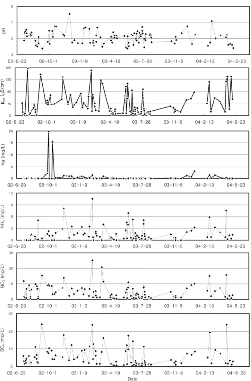
Fig. 1 compares the concentration variations of some of the major dissolved components in the meteoric water. The variation patterns of the conductivity (K
25), and three major air pollutants (NH
4, NO
3, and SO
4) are similar to one another, but significantly different from those of the rest.
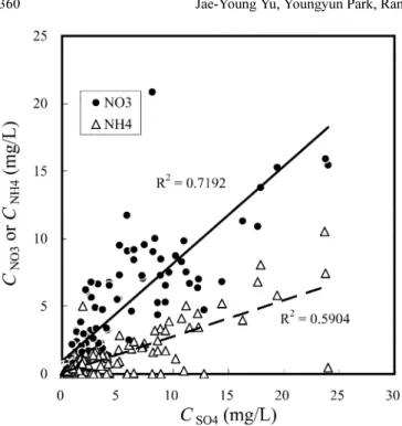
The correlation coefficients are fairly high among the three pollutants (Fig. 2), but those among other dissolved com- ponents are generally very low. It implies that the extent of air pollution is the key factor in controlling the chemistry of the meteoric water.
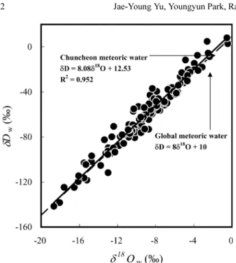
δD
wand δ
18O
wshow good correlation to each other, but both of them are poorly correlated with the air temperature (Fig. 3). Fig. 4 shows that the meteoric water aligns along a line parallel to the global meteoric water line, indicating that the water vapor formed at various locations and trans- ported to Chuncheon with little fractionation before deposition.
Fig. 1. Temporal variations of some of
the dissolved components in the mete-
oric water.
δ
34S
SO4and δ
18O
SO4were measured only for the meteoric water samples having enough amount of the dissolved SO
4to produce recoverable BaSO
4precipitate. Fig. 5 shows that δ
34S
SO4varies from 2.6 to 7.5‰ and its variation is inde- pendent of the concentration of the sulfate ( C
SO4), suggesting that the sources are not only variable but also inhomoge- neous (Krouse, 1980). Seasonal difference in δ
34S
SO4is not distinct. δ
34S of the coal being locally consumed has the values ranging from −4.5 to −0.7‰ with an average of
−2.7‰ (n=7), which is significantly different from δ
34S
SO4of the local meteoric water. Thus, the local sulfur emission from the coal combustion may insignificantly contribute to the local acid deposition.
One of the sources of SO
4in the meteoric water is the sea salt spray, whose fraction, A, in the total dissolved SO
4can be calculated from
(1) where C
Clis the concentration of the dissolved Cl in the meteoric water (Mizutani and Rafter, 1969). The rest of the dissolved sulfate may originate primarily from pollution sources. The calculated A values range from 0.006 to 0.15, but only a few are greater than 0.1. The isotopic composi- tions of non-sea-salt-spray SO
4(nssSO
4) can be calculated from δ
34S
SO4of meteoric water and sea salt spray together with the A values obtained from equation (1) (Yu and Park, 2004). The calculated δ
34S
SO4of nssSO
4are little different from that of total SO
4in the meteoric water.
δ
18O
SO4values range from 9.0 to 17.2‰ and show a little seasonal difference; the values in winter (from December to
February) are generally lower than those in spring (from March to May) (Fig. 6). δ
18O
SO4values are considerably scat- tered, especially at low C
SO4, but tend to increase with increas- ing C
SO4.
If there is little oxygen isotope fractionation or exchange during the oxidation and hydration of sulfide to form SO
4(from reactions (R1) to (R3)), δ
18O
SO4should be determined by 3:1 mixing of free oxygen and water oxygen, that is,
δ
18O
SO4= 0.75 δ
18O
a+ 0.25 δ
18O
w. (2) δ
18O
ahas been known to have a fairly constant value of 23.5‰ (Kroopnick and Craig, 1972). δ
18O
wvalues from this study vary from −16.1 to 0.5‰. With these oxygen iso- topic data, equation (2) gives δ
18O
SO4values between 13.6 and 17.5‰.
Fig. 6 indicates many of the measured δ
18O
SO4falls below the range defined by equation (2) (window A in Fig. 6), especially when C
SO4is low. This discrepancy is probably due to the isotope exchange between sulfite and water.
Lloyd (1968) compared the oxygen isotope exchange rate of sulfate-water with sulfite-water pair. The former is a function of pH and extremely slow at ambient pH. The latter is approximately 10
5times faster than the former. Stempvroot and Krouse (1980) confirmed that δ
18O
SO4was little affected by SO
4-H
2O exchange reaction. Holt et al. (1981) showed that δ
18O of sulfite was completely controlled by δ
18O
wand enriched by 24‰ with respect to δ
18O
win an equilibrium condition. Recently, Brunner et al. (2006) reported that the equilibrium fractionation at 23
oC produced the sulfite enriched by 11.5 and 7.9‰ with respect to the water at pH=7 and 8, respectively. The enrichment factor of Brunner et al. (2006) becomes fairly close to that of Holt et al.
(1981), if the values of Brunner et al (2006) are extrapo- lated to the pH of 4.5 corresponding to that of acid rain.
If SO
2is hydrated to form sulfite (reaction R2) and have enough time to be in equilibrium with water before further oxidation to sulfate (reaction R3), δ
18O of sulfite would be determined totally by the equilibrium fractionation between sulfite and water regardless of the amount of free oxygen constituting the sulfite. Then, if there is little oxygen isotope fractionation during the oxidation of sulfite, the resultant δ
18O
SO4should be given by
δ
18O
SO4= 0.75( δ
18O
w+ e
w) + 0.25 δ
18O
a, (3) where ε
wis the enrichment factor between sulfite and water given by Holt et al. (1981). Putting δ
18O
w= −16.1 to 0.5‰, ε
w=24‰, and δ
18O
a=23.5‰ into equation (3) gives δ
18O
SO4values ranging from 11.8 to 23.5‰. Fig. 6 shows that δ
18O
SO4limits calculated with equation (3) (window B in Fig. 6) enclose most of the measured δ
18O
SO4values of the samples, but there are still a few samples below the lower limit.
Moreover, the distribution of the δ
18O
SO4values are biased A C
Cl7.1 C
SO4---
=
Fig. 2. Variations of the concentrations of NH
4and NO
3as a func-
tion of the concentration of SO
4in the meteoric water.
Sulfur and oxygen isotopic compositions of the dissolved sulphate 361
towards the lower part of window B.
The biased distribution and the presence of outliers of δ
18O
SO4are possibly caused by the disequilibrium between sulfite and water, the non-zero oxygen isotopic fractionation during the sulfite oxidation, or the combination of the above two. Holt et al. (1981) performed numerous experiments of abiotic oxidation of sulfite and summarized the results with the following equation;
δ
18O
SO4= 0.75 δ
18O
w+ K. (4) where K varies depending on the experimental conditions.
From equations (3) and (4), the parameter K becomes
K = 0.75ε
w+ 0.25 δ
18O
a. (5)
Thus, the experiments by Holt et al. (1981) confirm that δ
18O
SO4is primarily determined by δ
18O
wand the fraction- ation of the oxygen isotopes between sulfite and water, where the fractionation occurs not necessarily under equi- librium condition.
It is worth noting that the lower C
SO4the meteoric water
shows, the lower δ
18O
SO4values and the wider concentra-
tion range the dissolved SO
4has. The low C
SO4often results
from the dilution by water. The longer the sulfur stays in the
air, the more water it would be diluted with and exchange
oxygen isotopes with. Thus, C
SO4may inversely propor-
tional to the residence time or the travel distance of sulfur
in the air and proportional to δ
18O
SO4. The wide variation of
δ
18O
SO4may result from isotopic inhomogeneity of the
Fig. 3. Temporal variations of the air
temperature and hydrogen and oxygen
isotopic compositions. The hydrogen
and oxygen isotopic compositions are
from Park et al. (2006).
remote water sources or variation in the extent of isotopic exchange depending on the physicochemical conditions of air mass. Fig. 7 shows that δ
18O
SO4has little correlation with δ
18O
w, which indicates that the variation not only in oxygen isotopic composition of the meteoric water but also in the extent of the isotopic exchange is responsible for the vari-
ation in δ
18O
SO4.
4. SUMMARY AND CONCLUSIONS
The sulfate in the meteoric water in Chuncheon, Korea comes primarily from anthropogenic sources. δ
34S
SO4of the Fig. 4. Variations of hydrogen isotopic composition as a function
of oxygen isotopic composition of the meteoric water.
Fig. 5. Sulfur isotopic compositions (δ
34S
SO4) plotted against the concentrations (C
SO4) of the dissolved sulfate in the meteoric water.
The spring, summer, fall and winter samples include those samples collected in March to May. June to August, September to November, and December to February, respectively.
Fig. 6. Variation of the oxygen isotopic compositions ( δ
18O
SO4) as a function of the concentrations ( C
SO4) of the dissolved sulfate in the meteoric water. Windows A and B are the oxygen isotopic compositional limits calculated by equation (2) and (3), respectively.
Fig. 7. Oxygen isotopic compositions of the dissolved sulfate
(δ
18O
SO4) plotted against those of water of the precipitation (δ
18O
w).
Sulfur and oxygen isotopic compositions of the dissolved sulphate 363 meteoric water collected from July 2002 to May 2004 var-
ies from 2.6 to 7.5‰ without a significant seasonal varia- tion. δ
34S of the sulfur in the coal being locally consumed has the values ranging from −4.5 to −0.7‰, indicating that the local coal consumption gives a minor contribution to the pollutant sulfur in the acid deposition of the area. The plot of δ
34S
SO4against C
SO4reveals that the sources of pollutant sulfur are not only variable but also inhomogeneous.
114)