논문 2014-51-7-2
Binary Particle Swarm Optimization 알고리즘 기반 분산 센서 노드 측위
( Distributed Sensor Node Localization Using a Binary Particle Swarm Optimization Algorithm )
이파 파티하*, 신 수 용***
( Ifa Fatihah and Soo Young Shin
ⓒ)
요 약
본 논문은 무선 센서 네트워크의 분산 분포되어 있는 센서 노드들의 측위를 위해 Binary Particle Swarm Optimization (BPSO) 알고리즘을 제안한다. 자신의 위치를 모르는 센서 노드들은 셋 이상의 인접한 앵커, 즉, 위치를 알고 있는 노드들로부터의 거리를 측정하여 측위를 수행한다. 이러한 과정이 반복하는 동안 측위를 수행한 센서 노드들은 나머지 노드들에 대하여 또 다른 앵커 역할을 수행한다. 성능 평가를 위해 기존의 PSO 알고리즘에 대비하여, BPSO를 이용한 측위 오류 및 계산 시간 성능을 매트랩 시뮬레이션을 통해 비교 분석하였다. 시뮬레이션 결과 PSO 기반의 측위가 상대적으로 더 정확한 결과를 보여준다. 대조적으로, BPSO 알고리즘은 분산되어 있는 센서 노드들의 위치 측위를 더 빠르게 수행한다. 추가적으로, 전송 범위와 초기 앵커 노드들의 수가 측위 성능에 미치는 영향에 대한 분석을 수행한다.
Abstract
This paper proposes a binary particle swarm optimization (BPSO) algorithm for distributed node localization in wireless sensor networks (WSNs). Each unknown node performs localization using the value of the measured distances from three or more neighboring anchors, i.e., nodes that know their location information. The node that is localized during the localization process is then used as another anchor for remaining nodes. The performances of particle swarm optimization (PSO) and BPSO in terms of localization error and computation time are compared by using simulations in Matlab. The simulation results indicate that PSO-based localization is more accurate. In contrast, BPSO algorithm performs faster for finding the location of unknown nodes for distributed localization. In addition, the effects of transmission range and number of anchor nodes on the localization error and computation time are investigated.
Keywords: BPSO, distributed localization, WSNs, localization error, computation time.
* 학생회원, 국립금오공과대학교 IT융복합학과 (Kumoh National Institute of Technology)
** 정회원, 국립금오공과대학교 전자공학부 (Kumoh National Institute of Technology)
ⓒ Corresponding Author(E-mail: [email protected])
※ 이 논문은 2013년도 정부(미래창조과학부)의 재원으 로 한국연구재단의 지원을 받아 수행된 기초연구사 업임(No. 2012R1A1A1009442).
접수일자: 2014년01월10일, 수정일자: 2014년04월16일 수정완료: 2014년06월23일
Ⅰ. Introduction
Wireless Sensor Networks (WSNs) consist of a huge number of wireless sensor nodes that are deployed over a certain area for data processing, sensing, and communications tasks. One of the main applications of WSNs is for monitoring different
physical or environmental conditions, such as sound, temperature, pressure, and movement.
Localization is the process of finding the locations of sensor nodes that are deployed randomly. To cope with the reported events in a timely fashion, knowing the locations of sensor nodes is critical for identifying and tracking where the events occur[1].
Generally, localization is performed by using the global positioning system (GPS). However, using GPS is not an effective solution owing to size, cost, and power consumption constraints and also because it is not applicable in certain scenarios[2]. Therefore, many WSN localization algorithms use special nodes called anchors to estimate the location of other nodes using a priori knowledge of the anchors' geographical coordinates while the other sensor nodes (unknown nodes) measure the distances or angles from anchors to estimate their positions by using an optimization algorithm that minimizes the localization error or by solving simultaneous equations[3].
In WSNs, a localization process requires additional communications and computations that consume additional energy. In a distributed architecture, the internode communication is limited to neighboring nodes only compared to the centralized case but more computational power and memory are required for localization in each sensor node. Hence, distributed localization offers a significant reduction in communication and computation overheads[4].
In this paper, we propose a bio-inspired binary particle swarm optimization (BPSO) for distributed localization in WSNs to reduce the computation power and computation time. For proving the effectiveness of the proposed algorithm, the performance of the proposed algorithm is compared with the distributed localization based on particle swarm optimization (PSO) in [5] and [6].
Our contributions can be summarized as follows:
1) We propose BPSO for distributed localization in WSNs to reduce the computation time. As measures of performance, both localization error and
computation time are used.
2) Our simulation results illustrate the tradeoff between localization error (accuracy) and computation time.
3) The effects of transmission range and the number of anchor nodes on the localization are investigated.
The rest of this paper is organized as follows:
Section Ⅱ discusses the related works; while Section
Ⅲ explains PSO and BPSO algorithms and also explains how the localization problem is addressed by using these algorithms. Section Ⅳ discusses the simulation results and in section V we present our conclusions.
Ⅱ. Related Work
PSO is a population-based stochastic optimization technique developed by Kennedy and Eberhart in 1995[7]. A summary of applications of PSO in WSN can be found in [8]. In [9], the authors proposed a localization method for WSNs with unknown nodes based on a priori information of location anchors using a PSO algorithm in centralized manner. In this approach, the distance measurements of neighboring anchor nodes are transferred to a central base station, that requires considerable communication, which may lead to congestion, delays, and also energy exhaustion.
In contrast, Kulkarni et al. proposed distributed iterative node localization in WSNs using a PSO algorithm[5~6]. An unknown node that has three or more anchors in its communication range runs PSO to minimize the localization error. The nodes that get localized serve as another anchors for other nodes.
This process continues iteratively, until either all the nodes get localized or no more nodes can be localized. This method does not require that each node transmit its distance measurement to a central node. In addition, using this method one can localize all nodes that have three localized nodes or anchors
in their communication range. However, localization based on PSO requires complex computations that require relatively large computation power and longer computation time.
Additionally, there is an extended version of PSO called BPSO. Unlike PSO, the BPSO algorithm has been used in binary discrete search spaces. The main advantage of BPSO is that it has a finite state of solutions, which can greatly reduce the computation time required for particle convergence compared to PSO[10].
Ⅲ. Proposed Algorithm
1. Basic PSO and BPSO
PSO is an optimization algorithm inspired by the social behavior of fish schooling or bird flocking.
Based on the problem of bird flocking, each bird is defined as a particle in the search space. The objective of the problem is to find the food. In this case, the search space represents the area around the food and the birds represent the particles in the search space. Each particle has its own distance from the food and it is defined as the cost function of the problem. Each particle has its own pbest (particle best) and among all the particles, there will be a bird (particle) whose location is the nearest to the food called gbest (global best). Based on PSO, the entire set of particles will therefore move toward the direction of the particle with gbest. In each iteration, the position and velocity of each particle are updated and the search for a new gbest will be executed.
This process is continuously iterated until the condition of termination is met.
Unlike PSO, the BPSO algorithm uses binary discrete search space. Kennedy and Eberhart have implemented BPSO to search in binary discrete search spaces[11]. By applying a sigmoid transformation to the velocity component, the velocities are forced to take values between 0 and 1, and the positions of the particles are either 0’s or 1’s.
Basically, the logical flow of PSO and that of BPSO are the same: Try to find pbest and gbest, and update the velocity and position of the particles. The only difference between the PSO and BPSO algorithms is in the equations used for defining the updates of velocity and position of each particle.
The velocity is updated by using the equation:
1
1 1( ) 2 2( )
id d
k k
id id best id best id
v
+ =wv
+c r p
−x
+c r g
−x (1)
where is the inertia weight of a particle, and
are the cognitive and social coefficients, while and are the random numbers in the range .
The equation to update the velocity in (1) is influenced by three components of acceleration. The inertia factor determines the confidence of a particle in its own movement unaffected by and . The cognitive coefficient, , determines how much a particle is influenced by the memory of its best solution and the social coefficient, , is an indication of the impact of the swarm on the particle.
The th dimension of the particle has the position and the velocity . The particles are initially assigned random positions and velocities within fixed boundaries, m in≤ ≤ m ax and
m in ≤ ≤ m ax. Then, the value of the position
and the velocity will be converted to binary number because the searching is done in binary space. Each particle in the swarm is evaluated by a cost function, . The cost function of a particle is determined from its position in the search space. In the BPSO algorithm, each particle has memory to store , the position where it had the lowest cost, and
, the position of the best particle in the population (or swarm).
The position of each particle is updated by using the equation:
( ) 1
1
idkk
id v
sigmoid v
e
−= + (2)
1, ( )
0,
k
k id
id
if rand sigmoid v
x otherwise
⎧ <
= ⎨ ⎩ (3)
By using the sigmoid function, the value of bit for the next position of is 1. This condition will occur if the random number is less than the value of the sigmoid function of the velocity at the current iteration and vice versa. In each iteration, velocities and positions of all particles are updated bit by bit to persuade them to achieve a lower cost.
2. Distributed Localization with BPSO Algorithm In this paper, we try to estimate the location of sensor nodes using distributed BPSO. The coordinate of unknown nodes, N, is estimated by using stationary anchors, M, which are assumed to know their own locations. Both unknown nodes and anchors are deployed randomly over a two-dimensional area.
Anchor nodes frequently transmit their coordinates and have a transmission radius of R. At the end of each iteration, the nodes that get localized will be used as additional anchors for unknown nodes. Each node is referred to as a localizable node if it is within the communication range from three or more neighboring anchors or any localized nodes, ≥ . Each localizable node estimates its distance from each of its neighboring anchors through:
2 2
( ) ( )
i i i
d
=x x
− +y y
−(4)
2 2 2
1
1 ˆ
( , ) M ( ( i) ( i) i)
i
f x y x x y y d
M =
=
∑
− + − −(5)
where is the location of the unknown nodes and
is the location of anchors. The actual distance, in (4) is the Euclidean distance between two nodes. Both PSO and BPSO will find the
coordinates that minimize the cost function, , that represents the localization error in the WSN.
Equation (5) is used in the calculation to determine the error, which is defined as the difference between the estimated distance and the actual distance of the nodes, where is the value of obtained from a noisy range measurements, .
The pseudocode of BPSO algorithm for minimization of a cost function is given in Algorithm 1.
3. Communication Model
Determining the distances between sensor nodes can be classified into three categories: angle of arrival (AoA) measurements, time of arrival (ToA) or time difference of arrival (TDoA) measurements, and the received signal strength (RSS) measurements.
In this paper, the received signal strength
indication (RSSI) approach is used because of its simple implementation in the hardware and also low cost[12]. Since the nodes in the network communicate with their neighbors only, the RSSI signal can be measured without additional energy consumption.
The neighboring nodes of the anchor estimate their distance from the anchor by measuring the RSSI of the broadcast signal. A node estimates distances from each of the anchors if it receives a broadcast signal from at least three anchors. In general, the RSSI value increases if the anchor node is closer to the sensor node and vice versa in both indoor and outdoor environments. Measured RSSI values are known to fluctuate over time[13]. Hence, to reduce the estimation error, an optimization technique is required. The distance from the anchor to unknown node is calculated using:
0
10 (logD)
RSSI P n X
D σ
= − × +
(6)
where is the received power at the reference distance, , is the path loss index, is the nodes distance, and is a zero mean Gaussian random variable, .
Ⅳ. Simulation Results and Discussion
To evaluate the performance of the proposed algorithms, we used Matlab for simulations. The parameters used for localization are listed in Table 1 and the parameters for PSO and BPSO algorithms are listed in Table 2.
In this paper, localization error and computation
Parameter Value
Sensor Field Size 100 m x 100 m Stationary Anchor Nodes, M 10
Unknown Nodes, N 50
Transmission Range, R 25 m 표 1. 측위를 위한 시뮬레이션 매개 변수 Table 1. Simulation parameters for localization.
Parameter Value
Maximum Iteration, m ax 150 Inertia Weight, 0.7 Acceleration Constant, 2.0 Random Numbers, [0,1]
Particle Positions min max
Particle Velocities min max
표 2. 제안 된 알고리즘에 대한 시뮬레이션 매개 변 수
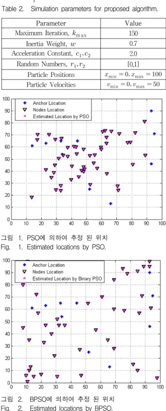
Table 2. Simulation parameters for proposed algorithm.
그림 1. PSO에 의하여 추정 된 위치 Fig. 1. Estimated locations by PSO.
그림 2. BPSO에 의하여 추정 된 위치 Fig. 2. Estimated locations by BPSO.
time are used for the performance metrics. The average localization error determines how accurate the localization is expected to be while the computation time determines how quickly the
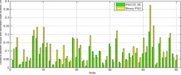
그림 3. PSO와 BPSO에 의한 실제 및 예상 측위간 거리 차이
Fig. 3. Distance between actual and estimated node location by PSO and BPSO.
localization can be done.
The actual location of nodes and anchors and the coordinates of the nodes estimated by PSO and BPSO algorithms are shown in Fig. 1 and Fig. 2, respectively. The deployment of anchor nodes for both algorithms is identical for comparison purposes.
The simulation results of both PSO and BPSO algorithms show that all 50 unknown nodes can be localized inside the sensor field.
The average localization error is defined as the total error between the node location and the estimated location obtained by using the algorithm divided by the total number of unknown nodes, N.
Fig. 3 shows a comparison for both algorithms in terms of localization error for each unknown node.
From Fig. 3, the accuracy is seen to be better in PSO but the error difference between PSO and BPSO is less than 34.31% on average.
To compare the performance of the proposed algorithms, the computation time needed in the simulation for each algorithm is also evaluated.
Although the computation time depends on the network size, computational power, and the complexity of the localization method, it could be assumed that longer computation time means more energy consumption without loss of generality.
Algorithm Average Localization Error, m
Computation Time, s
PSO 0.0809 361.6185
BPSO 0.1144 201.1747
표 3. PSO와 BPSO 성능 비교
Table 3. Performance Comparison between PSO and BPSO.
In our paper, we run the simulation for 10 times only (using the same computer) and calculate the average value for both localization error and computation time from a statistical analysis. The details of performance are summarized in Table 3.
From Table 3, it can be seen that the BPSO algorithm suffers from a higher average localization error but uses less computation time compared to the PSO algorithm.
In PSO, the update rule uses the current position of the particle and the velocity vector to determine the movement of the particle in space[14]. However, in BPSO, the next value for the bit is independent of the current value of that bit and it is solely updated by using the velocity vector. That is why the BPSO algorithm produces lower localization accuracy compared to PSO. Additionally, the required computation time in BPSO is small compared to PSO because the searching is done in binary space.
In summary, although the PSO determines the node coordinates more accurately, the BPSO does so more quickly. In detail, the simulation results showed that the proposed algorithm reduced the computation time required for the localization by 57.02% while increasing the localization error by 34.31%.
As computation time is decreased, power consumption is also reduced. As we know, the main drawback of WSNs is power consumption or energy constraint because of the impracticality of recharging or changing the battery. From the simulation results, as computation time is decreased, power consumption is also reduced. Hence, the proposed algorithm can provide a good solution for the main weakness of WSNs.
Next, further analysis related to transmission range and number of anchor nodes are done to investigate the effect of these parameters on the localization error.
In general, better localization performance is expected with a higher transmission range[15]. Therefore, the transmission range is changed by increasing the value of R from Table 1 to obtain better localization performance. Increasing the transmission range reduces the localization error for both PSO and BPSO algorithms as shown in Fig. 4.
When an anchor node decreases its transmission range, there could be coverage holes between neighboring anchors. Hence, there are chances that
그림 4. 전송 범위 대 측위 오류
Fig. 4. Localization error vs. transmission range.
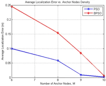
그림 5. 앵커 노드의 수 대 측위 오류
Fig. 5. Localization Error vs. Number of Anchor Nodes.
anchor nodes might lose the unknown node and fail to locate it. As a result, localization error will increase with a lower transmission range. In contrast, localization error is reduced with a higher value of R because more anchors will cover the unknown nodes, resulting in more accurate localization.
If unknown nodes cannot measure the distances from three or more anchors, localization itself is impossible. In such a situation, the only option is to increase the number of anchor nodes in the network to increase the coverage[16]. Therefore, the number of anchor nodes, M, is changed for evaluating the effect of M on the localization performance. The performance of the localization algorithm as a function of anchor nodes is shown in Fig. 5.
As the results clearly indicate, increasing the number of anchor nodes in the network can substantially improve localization accuracy with lower localization error. The algorithms will produce more errors with fewer anchor nodes because an unknown node needs to engage in more distance measurements for location estimation process to find its locations with respect to anchor nodes. Therefore, the unknown node is more vulnerable to the probability of error. Hence, the probability of error accumulation is reduced with the growing network size for both PSO and BPSO algorithms.
V. Conclusion
In this paper, we proposed a binary particle swarm optimization algorithm for distributed node localization. Each unknown node performs localization under the measurement of distances from three or more neighboring anchors. The localized node during iteration is then used as another anchor for remaining nodes. The distance from the anchor to the unknown node is calculated by using the received signal strength indication. To prove the effectiveness, the performance of the proposed algorithm was compared to that with PSO. As measures of performance, localization error and computation time are used during simulations in Matlab. Simulation results showed a tradeoff with the proposed algorithms: PSO determines the node coordinates more accurately, but BPSO does so more quickly. Reducing computation time for localization can save energy and extend the lifetime of the WSN. In addition, some further analysis related to transmission range and number of anchor nodes are done to investigate the effect of these parameters on the performance of nodes localization.
REFERENCES
[1] K.-S. Low, H. Nguyen, and H. Guo, “A particle swarm optimization approach for the localization of a wireless sensor network,” in IEEE International Symposium on Industrial Electronics, pp. 1820-1825, 2008.
[2] Kwanghee Lee, Ik-Su Seo, and Dong Seog Han,
“Target Localization Using Underwater Objects in Multistatic Sonar,” in Journal of The Institute of Electronics and Information Engineers, Vol.
51, no. 2, pp. 381-387, 2014.
[3] Jin-Gwan, Min-A Jung, Kyoung-Ho Kim, and Seong-Ro Lee, “WSN Data Visualization using Augmented Reality,” in Journal of The Institute of Electronics and Information Engineers, Vol.
50, no. 12, pp. 3045-3054, 2013.
[4] Q. Shi, C. He, H. Chen, and L. Jiang,
“Distributed wireless sensor network localization
via sequential greedy optimization algorithm,” in IEEE Transactions on Signal Processing, Vol.
58, no. 6, pp. 3328-3340, 2010.
[5] R. Kulkarni, G. Venayagamoorthy, and M.
Cheng, “Bio-inspired node localization in wireless sensor networks,” in IEEE International Conference on Systems, Man and Cybernetics, pp. 205-210, 2009.
[6] R. Kulkarni and G. Venayagamoorthy,
“Bio-inspired algorithms for autonomous deployment and localization of sensor nodes,” in IEEE Transactions on Systems, Man, and Cybernetics, Part C: Applications and Reviews, Vol. 40, no. 6, pp. 663-675, 2010.
[7] J. Kennedy and R. Eberhart, “Particle swarm optimization,” in Proceedings of IEEE International Conference on Neural Networks, Vol. 4, pp. 1942-1948, 1995.
[8] R. Kulkarni and G. Venayagamoorthy, “Particle swarm optimization in wireless-sensor networks:
A brief survey,” in IEEE Transactions on Systems, Man, and Cybernetics, Part C:
Applications and Reviews, Vol. 41, no. 2, pp.
262-267, 2011.
[9] A. Gopakumar and L. Jacob, “Localization in wireless sensor networks using particle swarm optimization,” in IET International Conference on Wireless, Mobile and Multimedia Networks, pp.
227-230, 2008.
[10] Z. Yusof, T. Z. Hong, A. Abidin, M. Salam, A.
Adam, K. Khalil, J. Mukred, N. Shaikh-Husin, and Z. Ibrahim, “A two-step binary particle swarm optimization approach for routing in vlsi with iterative rlc delay model,” in Third International Conference on Computational Intelligence, Modelling and Simulation, pp. 63-67, 2011.
[11] J. Kennedy and R. Eberhart, “A discrete binary version of the particle swarm algorithm,” in IEEE International Conference on Systems, Man, and Cybernetics, Vol. 5, pp. 4104-4108, 1997.
[12] N. Patwari, J. Ash, S. Kyperountas, A. Hero, R.
Moses, and N. Correal, “Locating the nodes:
cooperative localization in wireless sensor networks,” in IEEE Signal Processing Magazine, Vol. 22, no. 4, pp. 54-69, 2005.
[13] P. Sahu, E.-K. Wu, and J. Sahoo, “Durt: Dual rssi trend based localization for wireless sensor networks,” in IEEE Sensors Journal, Vol. 13, no.
8, pp. 3115-3123, 2013.
저 자 소 개 이파 파티하(학생회원)
2012년 University of Technology Malaysia 졸업(학사).
2012년~현재 국립금오공과대학교 IT융복합학과 석사과정.
<주관심분야 : 무선통신, 생태계 모방 알고리즘, 에너지 효율화, etc.>
신 수 용(정회원)
1999년 서울대학교 전기공학부 졸업 (학사).
2001년 서울대학교 대학원 전기공학부 졸업(석사).
2006년 서울대학교 대학원 전기 컴퓨터공학부 졸업(박사).
2010년~현재 국립금오공과대학교 전자공학부 교수.
<주관심분야 : 무선통신, 3G/4G, WLAN/WPAN /WBAN, 산업용통신망, 실시간시스템, etc.>
[14] M. Khanesar, M. Teshnehlab, and M.
Shoorehdeli, “A novel binary particle swarm optimization,” in Mediterranean Conference on Control Automation, pp. 1-6, 2007.
[15] S. Chaudhary, A. Bashir, and M.-S. Park,
“[etctr] efficient target localization by controlling the transmission range in wireless sensor networks,” in Fourth International Conference on Networked Computing and Advanced Information Management, Vol. 1, pp.
3-7, 2008.
[16] E. Niewiadomska-Szynkiewicz, “Localization in wireless sensor networks: Classification and evaluation of techniques,” pp. 281-297, June 2012.