Efficient Triangulation Algorithm for Constructing the Model Surface from the Interpolation of Irregularly-Spaced Laser Scanned Data
Howoong Shon
Dept. of Civil and Geotechnical Engineering, Paichai University, Korea
ABSTRACT A discussion of a method has been used with success in terrain modelling to estimate the height at any point on the land surface from irregularly distributed samples. The special requirements of terrain modelling are discussed as well as a detailed description of the algorithm and an example of its application.
Key words triangulation, interpolation, surface model, laser scan data
1. Introduction
There are a number of possible techniques that can be used for surface interpolation, that is, estimating the height at a point given nearby sample heights. Some of the more com- mon methods are natural neighbour interpolation, surface patches, quadratic surfaces, polynomial interpolation, spline interpolation, and Delauney Triangulation an im- plementation of which is described here. Some such inter- polation is often required in the display of empirical data, for example, terrain modelling where elevation samples are obtained from surveys, meteorology where data is collected from weather stations, regional planning using data collec- tion stations, and mesh generation for finite element analysis.
This paper discusses a technique suitable for terrain mod- elling but also for other applications which have the follow- ing characteristics :
○ There are regions of high and low sample density. For example, in terrain modelling there will generally be a low sample density inside bodies of water and a high sam- ple density in the areas of particular interest.
○ There may be discontinuities in the surface resulting in samples very close to each other on the sample plane but of wildly differing height values. These may be natural structures as cliffs and river banks or man-made dis- continuities like retaining walls. Most smoothing meth- ods do not handle these cases very well especially those
based on polygonal functions where surface overshoot, oscillation and general instability occurs.
○ the samples often lie along contours. These may be de- rived from existing contour maps or from the paths taken by a survey team. This is another aspect of differing sam- ple densities. Along the sampling curves there is a high sampling density but perpendicular to the path there are no samples until the next path is reached.
○ A large number of samples will often need to be handled.
The time needs to increase modestly as the number of samples increases for a technique to be suitable. Typical sample numbers may be from 100 to 100,000. Such large numbers of samples are particularly common when auto- mated sampling methods are employed.
○ Samples are often obtained in an incremental procedure.
An initial sample may be collected and analyzed, the areas of interest can then be sampled at a higher density.
It is advantageous to be able to add the new points to the surface obtained so far thus refining the current surface definition as opposed to recomputing the surface from scratch from the combined set of data points.
○ The algorithm should be such that it can be run on desktop computers where large amounts of memory, disk space or fast processors can not be assumed.
The technique to be discussed has been used for terrain
modelling with success, it copes with the above aspects of
many terrain data sets, and it readily lends itself to grid and
contour generation as well as 3D rendering.
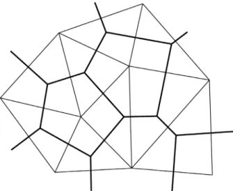
Fig. 1 Delauney triangles (thin lines) and associated Direchlet Tesselations (thick lines) for nine generating points. Triangle edges are perpendicular bisectors of the tile edges. Points within a tile are closer to the tile's generating point than to any other generating point.
2. Triangulation
Triangulation involves creating from the sample points a set of non-overlapping triangularly bounded facets, the vertices of the triangles are the input sample points. There are a number of triangulation algorithms that may be advo- cated, the more popular algorithms are the radial sweep method and the Watson algorithm which implement Delaunay triangulation.
The Delauney triangulation is closely related geometri- cally to the Direchlet tesselation also known as the Voronoi or Theissen tesselations (Fig. 1). These tesselations split the plane into a number of polygonal regions called tiles. Each tile has one sample point in its interior called a generating point. All other points inside the polygonal tile are closer to the generating point than to any other. The Delauney trian- gulation is created by connecting all generating points which share a common tile edge. Thus formed, the triangle edges are perpendicular bisectors of the tile edges.
Such a triangulation has many desirable features. It can be shown that a convex equilateral formed by two adjacent triangles has a greater minimum internal angle than if the equilateral was formed another way. In this sense the tri- angles are as equilateral as possible, thin wedge shaped tri- angles are avoided.
The triangulation is unique (independent of the order in
which the sample points are ordered) for all but trivial cases.
One such case is if four points lie on the corners of a rectangle, they may be triangulated in one of two ways. These situation occur rarely in real data but if uniqueness is important then a straightforward solution is to perturb one or more of the vertices on the offending rectangle.
One particular situation where many other techniques perform poorly is when there is a mixture of regions of high and low density sampling. Triangulation based methods honor this situation by giving a large number of triangles and hence more detail to the highly sampled regions and large triangles, less detail, to the regions with a few samples.
Discontinuities are handled quite naturally. The surface can have a discontinuity as narrow as the sampling process permits, it simply results in near vertical triangular facets.
Note however that unless special action is taken there can not be two samples at precisely the same point on the sample plane but with different heights. This can occur with discrete digitizer when digitizing near discontinuities. A perturba- tion of the sample point in the correct direction is usually a satisfactory solution to this problem.
An algorithm to implement triangulation can be quite ef- ficient and thus suitable for areas with a large number of samples. Furthermore if further samples are obtained at a later date they can be added to the already existing triangu- lation without having to triangulate all the samples plus the extra samples. This makes it possible to efficiently perform a successive refinement on those areas where more detailed information is required.
The planar surfaces formed may be used directly as facets
making up the surface or they may be used to produce sam-
ples on a regular grid. Given a list of triangular bounded fac-
ets it is simply a matter of finding the facet whose projection
onto the sample plane encloses the point to be estimated. The
intersection of the facet plane at the grid point is the estimate
of the height. Another method of estimating the points on
a grid is to use the Direchlet tesselations instead of the trian-
gular facets. This avoids the cone shaped peaks about local
minima and maxima which the first method tends to
generate. It is intuitively more appealing because the tesse-
lations correspond to an area of influence about the sample
points. Contour maps can be generated directly from the tri-
angular facets or from the samples distributed on a rec-
tangular grid. Generating smooth surfaces if that is required
is also generally easier if gridded data is available.
3. Algorithm
At any stage of the triangulation process one has an exist- ing triangular mesh and a sample point to add to that mesh.
The process is initiated by generating a supertriangle, an arti- ficial triangle which encompasses all the points. At the end of the triangulation process any triangles which share edges with the supertriangle are deleted from the triangle list:
1. (Fig. 2a) : All the triangles whose circumcircle encloses the point to be added are identified, the outside edges of those triangles form an enclosing polygon. (The circum- circle of a triangle is the circle which has the three vertices of the triangle lying on its circumference).
2. (Fig. 2b) : The triangles in the enclosing polygon are de- leted and new triangles are formed between the point to be added and each outside edge of the enclosing polygon.
3. (Fig. 2c) : After each point is added there is a net gain of two triangles. Thus the total number of triangles is twice the number of sample points. (This includes the super- triangle, when the triangles sharing edges with the super- triangle are deleted at the end the exact number of tri- angles will be less than twice the number of vertices, the exact number depends on the sample point distribution) The triangulation algorithm may be described in pseu- do-code as follows:
subroutine triangulate input : vertex list output : triangle list initialize the triangle list determine the supertriangle
add supertriangle vertices to the end of the vertex list add the supertriangle to the triangle list
for each sample point in the vertex list initialize the edge buffer
for each triangle currently in the triangle list calculate the triangle circumcircle center and radius if the point lies in the triangle circumcircle then add the three triangle edges to the edge buffer remove the triangle from the triangle list endif
endfor
delete all doubly specified edges from the edge buffer this leaves the edges of the enclosing polygon only add to the triangle list all triangles formed between
the point
and the edges of the enclosing polygon endfor
remove any triangles from the triangle list that use the supertriangle vertices
remove the supertriangle vertices from the vertex list end
The above can be refined in a number of ways to make it more efficient. The most significant improvement is to pre- sort the sample points by one coordinate, the coordinate used should be the one with the greatest range of samples. If the x axis is used for presorting then as soon as the x component of the distance from the current point to the circumcircle cen- ter is greater than the circumcircle radius, that triangle need never be considered for later points, as further points will never again be on the interior of that triangles circumcircle.
With the above improvement the algorithm presented here increases with the number of points as approximately O(N^1.5).
The time taken is relatively independent of the input sam- ple distribution, a maximum of 25% variation in execution times has been noticed for a wide range of naturally occur- ring distributions as well as special cases such as normal, uniform, contour and grid distributions.
The algorithm does not require a large amount of internal storage. The algorithm only requires one internal array and that is a logical array of flags for identifying those triangles that no longer need be considered. If memory is available another speed improvement is to save the circumcircle cen- ter and radius for each triangle as it is generated instead of recalculating them for each added point. It should be noted that if sufficient memory is available for the above and other speed enhancements then the increase in execution time is almost a linear function of the number of points.
An example where the triangulation algorithm described above is used to model land surfaces is given in Figs. 3 and 4.
4. Conclusions
A discussion of a method has been used with success in terrain modelling to estimate the height at any point on the land surface from irregularly distributed samples.
Triangulation involves creating from the sample points
Fig. 2(a) New sample point to be added to existing triangular mesh.
Fig. 2(b) Triangles whose circumcircle include the new point form an enclosing polygon.
Fig. 2(c) New triangular polygons formed from new point to the outside edges of the enclosing polygon.
Fig. 4 A perspective wire frame of a gridded surface obtained from a triangulated mesh.
Fig. 3 The result of triangulating spot heights.
a set of non-overlapping triangularly bounded facets, the vertices of the triangles are the input sample points.
The Delauney triangulation is closely related geometri- cally to the Direchlet tesselation also known as the Voronoi or Theissen tesselations. These tesselations split the plane into a number of polygonal regions. Each tile has one sample point in its interior called a generating point. All other points inside the polygonal tile are closer to the generating point than to any other. The Delauney triangulation is created by connecting all generating points which share a common
tile edge. Thus formed, the triangle edges are perpendicular bisectors of the tile edges.
The technique to be discussed has been used for terrain modelling with success, it copes with the above aspects of many terrain data sets, and it readily lends itself to grid and contour generation as well as 3D rendering.
References
Akima, N., 1978, A Method of Bivariate Interpolation and Smooth Surface Fitting for Irregularily Distributed Data Points.ACM Transactions on mathematical Software. V. 4, No.
1, 56-76.
Barnhill, R.E., 1975, Gregory, J.A. Polynomial Interpolation to Boundary Data on Triangles Mathematics of Computation, No. 29, 238-245.
Bourke, P.D. 1987, A Contouring Subroutine. BYTE Magazine, June, 456-467.
Green P. J., and Sibson R., 1981, Computing Dirichlet Tesselations in the Plane. The Computer Journal, No. 24, 127-132.
Holroyd, M.T., and Bhattacharya, B.K., 1970, Automatic Contouring of Geophysical Data Using Bicubic Spline Interpolation. Dept. of Energy, Mines, and Resources Publi- cations. Geological Survey of Canada, 128p.
Ilfick, M. H., 1979, Contouring by Use of a Triangular Mesh.
Cartographic Journal, 24-28.
McCullagh, M.J., 1981, Creation of Smooth Contours Over Irregularly Distributed Data Using Local Surface Patches.
Geographical Analysis, V. 13, No. 1, 34-41.
Mirante, A., and Weingarten, N., 1982, The Radial Sweep Algorithm for Constructing Triangulated Irregular Networks.
IEEE Computer Graphics and Applications, V. 2, No. 3, 289- 293.
Sibson, R. A, 1981, Brief History of Natural Neighbour Inter- polation. In Barnett, V. Interpreting Multivariate Data, John Wiley & Sons, New York, 367-388.
Sloan, S. W. and Houlsby, G.T., 1984, An Implementation of Watson's Algorithm for Computing 2-D Delauney Triangu- lations. Advanced Engineering Software, V. 6, No. 4, 189- 192.
Petrie, G. and Kennie, T.J.M, 1987, Terrain modelling in Survey and Civil Engineering. Computer Aided Design, V. 19, No. 4, 289-296.
Yoeli, P., 1977, Computer Executed Interpolation of Contours into Arrays of Randomly Distributed Height Points. Cartographer Journal, V. 14, No. 2, 67-77.