Comparison of two sampling intervals and three sampling intervals VSI charts for monitoring both
means and variances †
Duk-Joon Chang 1
1 Department of Statistics, Changwon National University
Received 5 June 2015, revised 11 June 2015, accepted 15 June 2015
Abstract
In industrial quality control, when engineers use VSI control procedure they should consider both required time to signal and switching behaviors together in the case of production process changed. Up to the present, many researchers have studied fixed sampling interval (FSI) chart and variable sampling interval (VSI) chart in the points of average number of samples to signal (ANSS) and average time to signal (ATS).
However, ANSS and ATS do not provide any switching information between different sampling intervals of VSI schemes. In this study, performances of two sampling inter- vals VSI chart and three sampling intervals VSI chart are evaluated and compared.
The numerical results show that ANSS and ATS values of two sampling intervals VSI chart and three sampling interval VSI chart are similar regardless the amount of shifts.
However, the values of switching behaviors including ANSW are less efficient in three sampling intervals VSI charts than in two sampling intervals VSI chart.
Keywords: ANSW, ATS, required time to signal, switching behavior, VSI chart.
1. Introduction
Control chart is widely used tool to display sample data from a production process for quick determining whether a process is in control state or not, for bringing an out of control process into control state, and for monitoring a process to make sure that it stays in control state. When the control chart signals that an assignable cause is present, then a rectifying action is taken to remove the assignable cause and bring the process back into in control state.
The usual and traditional practice in using a control chart to monitor a production process is to take samples at fixed time length sampling intervals and the properties of control charts have been developed when the sampling interval between samples is fixed.
The properties of control procedures when the sampling interval between samples is not fixed but rather depends on what is being observed in the current samples were investigated by Reynolds et al. (1990), Amin and Miller (1993). The basic idea of VSI procedure is that
† This research is financially supported by Changwon National University in 2013-2014.
1
Professor, Department of Statistics, Changwon National University, Changwon 641-773, Korea.
E-mail: [email protected]
the sampling interval should be short when a chart statistic falls close to a control limit, and should be long if the chart statistic is close to target since there is no indication of a change in the process.
Theoretical and numerical comparisons between FSI procedures and VSI procedures show that the VSI procedures are substantially efficient in terms of ATS when the ANSS values of both types of charts are held equal. Cui and Reynolds (1988) considered VSI Shewhart X-chart with runs rules using Markov chain method and Markov chain method for multi- variate EWMA chart can be referred from Chang et al. (2003). Multivariate process control procedures were studied by Jeong and Cho (2012) and Park and Cho (2013).
Frequent switching between different sampling intervals can be a complicating factor in application of VSI control chart. Hence it is necessary to keep as small the number of switches as possible for the different sampling intervals either the process in control state or not when VSI procedure is applied. The ANSS and the ATS do not directly provide information on how frequently switches are made, and so it is necessary to provide new quantities which measure the frequency of switching in VSI procedures.
Many studies on the ability of a VSI chart have been focused on the length of time re- quired for the chart to signal like ATS and ANSS when the process is changed. However, major shortcoming of VSI procedure in industry is that frequent switching between dif- ferent intervals d 1 , d 2 , · · · , d k requires more cost and effort to administer the process than corresponding FSI procedure.
Amin and Letsinger (1991) described general procedures for combining VSI feature and examined switching behavior and runs rules for switching between different sampling in- tervals. They also presented that the average number of switches to signal (ANSW) of the CUSUM and EWMA charts exists far fewer than the Shewhart charts. Bai and Lee (2002) investigated three switching rules to the ¯ X control charts and the expressions of the ATS and ANSW were derived with Markov chain approach.
Up to the present, studies of three sampling intervals VSI chart are hard to find, and studies comparing the efficiencies between two sampling intervals VSI chart and three sampling intervals VSI chart are also hard to find.
This paper mainly focused on the performances of ATS and switching behaviors between different sampling intervals for simultaneously monitoring both means and variances of mul- tivariate normal process. In addition, this research suggests some criteria that a quality engineer in industry should consider before selecting one of the two procedures, two sam- pling interval VSI chart and three sampling interval VSI chart.
In this paper we assumed that the sequential samples are independent, but one could note that the production processes are inherently time-dependent. This time-dependent problem can be studied in future works.
2. Control statistics for means and variances
Many situations in industrial quality control procedures usually involve a vector of quality
measurements of p (p ≥ 2) correlated random variables X 1 , X 2 , · · · , X p rather than a single
variable. Therefore we assume that the quality of a product has p quality variables repre-
sented by the random vector X 0 = (X 1 , X 2 , · · · , X p ). We assume that the production process
of interest has p quality variables whose distribution are multivariate normal N p (µ, Σ), and
(µ 0 , Σ 0 ) is the known target process parameters for (µ, Σ).
At each sampling time i (i = 1, 2, · · · ), we take a sequence of random vector X 0 i = (X 0 i1 , X 0 i2 , · · · , X 0 ∈ ) where X 0 ij = (X ij1 , X ij2 , · · · , X ijp ). Thus X i is an np × 1 column vector.
Then the jkth element X ijk of X i is the jth observation for kth quality variable at every sampling time i (j = 1, 2, · · · , n; k = 1, 2, · · · , p). It also be assumed that the sequential ob- servation vectors between and within samples are independent and identically distributed.
To monitor both mean µ and variance σ 2 of a single quality variable, Reynolds and Ghosh (1981) proposed an obvious method for simultaneously monitoring µ and σ 2 to use the control statistic
M V i =
n
P
j=1
(X ij − µ 0 ) 2
σ 0 2 = n(X i − µ 0 ) 2 σ 0 2 +
n
P
j=1
(X ij − X i ) 2
σ 2 0 (2.1)
and the univariate Shewhart chart in (2.1) signals if M V i ≥ χ 2 1−α (n). Extending the control statistic M V i to multivariate case, we obtain the control statistic D i for multivariate chart
D i =
n
X
j=1
(X ij − µ
0 ) 0 Σ −1 0 (X ij − µ
0 ). (2.2)
By simple calculation we can obtain
D i = Z i 2 + V i , where Z i 2 = n(X i −µ
0 ) 0 Σ −1 0 (X i −µ
0 ), V i = tr(A i Σ −1 0 ) and A i = P n
j=1 (X ij −X i )(X ij − ¯ X i ) 0 . If the production process is in control state, the statistic D i has a chi-squared distribution with np degrees of freedom. Alt (1984) used Z i 2 for controlling the mean vector µ and some researchers used V i for monitoring the variance-covariance matrix Σ. Note that the multivariate statistics Z i 2 and V i are independent and when µ = µ 0 and Σ = Σ 0 , then Z i 2 ∼ χ 2 (p) and V i ∼ χ 2 ((n − 1)p), respectively.
When the production process has shifted from target mean vector µ
0 to µ, D i and Z i 2 has a non-central chi-squared distribution with noncentrality parameter τ 2 = n(µ − µ 0 ) 0 Σ −1 0 (µ − µ 0 ), and np and p degrees of freedom respectively. The noncentrality parameter associated with χ 2 is λ 2 (µ) = n(µ − µ 0 ) 0 Σ −1 0 (µ − µ 0 ) and the scale λ 2 (µ) is often used to represent a measure of the distance of µ from µ
0 . And, the ANSS values of the multivariate Shewhart χ 2 chart depend on only through the statistical distance d = q
n(µ − µ
0)
0Σ
−10(µ − µ
0) . Therefore, it is possible to consider the ANSS as a function of statistical distance d.
When the process shifts on Σ or both µ and Σ, then it is difficult to obtain the exact distribution of D i and V i . For this reason, it is necessary to use computer simulation in order to obtain various performances of multivariate chart including switching behavior, ATS and so on.
To investigate and compare the performances of considered multivariate Shewhart control chart, there are various forms in which the shifts could take place on both means and/or variances. But for simplicity in this study, we consider the following typical types of shifts and evaluate the performances of such types in the process. The types of shift in the process parameters when the process is out of control for comparison can be stated as follows :
(1) shift in means : M i - µ 1 in µ shifted with τ 2 = (0.5i) 2
(2) shift in variances : V i - σ 10 in Σ 0 is increased to (1.0 + 0.05i) (3) shift in means and variances : (M i , V i ).
3. VSI charts with two and three sampling intervals
The problem of determining sampling plans with variable sampling intervals was first investigated by Arnold (1970). Extension of Arnold’s study presented by Smeach and Jerni- gan (1977). They derived equations for the variance of the sample size and approximation schemes that could enhance the implementation of this sampling procedure.
Reynolds et al. (1988) considered the properties and details of the application of VSI feature to the Shewhart X-chart and showed that VSI feature substancially reduce the average time to signal. Reynolds and Arnold (1989) and Reynolds (1989) investigated the theoretical aspects of one- and two-sided VSI Shewhart charts in detail and showed that the use of two sampling intervals spaced as apart as possible is optimal in terms of reduction of the time to signal when the process is changed.
The sampling intervals are not constant in VSI procedures, and samples will not taken irregular time intervals. This erratic behaviors could complicate the process operation for engineers who have to control the production process. Thus it would be desirable to keep the number of switches between different sampling intervals to a minimum without reducing the abllity of VSI procedures to detect shifts in the process.
Shewhart χ 2 chart for monitoring both means and variances in (2.2) with fixed sampling interval (FSI) signals whenever χ 2 i > χ α (q), and the ANSS of this chart can be calculated as 1/q where q denotes the probability that the chart statistic χ 2 i exceeds the upper control limit (UCL) χ α (q).
For the two sampling intervals VSI chart, suppose that the two sampling intervals d 1 is used whenχ 2 ∈ (g, h]
d 2 is used whenχ 2 ∈ (0, g],
where d 1 < d 2 . The design parameters g, h are chosen to give specified ANSS and ATS values when the process is in control state.
For the three sampling intervals VSI chart, suppose that the three sampling intervals d 1 is used when χ 2 ∈ (g 2 , h]
d 2 is used whenχ 2 ∈ (g 1 , g 2 ] (3.1) d 3 is used whenχ 2 ∈ (0, g 1 ],
where d 1 < d 2 < d 3 . The design parameters h, g, g 1 , g 2 are chosen to give specified ANSS and ATS values when the process is in control state.
If we let T be the time to signal, and R i be the sampling interval used before the ith sample is taken, then T = P N
i=1 R i where N is the average number of samples to signal.
Note that the distribution of each R i is the conditional distribution of sampling interval function d(X i ) given that there is no signal at the previous sample.
For simplicity in this paper, we assume that the chart is started at time 0 and that R 1 ,
the interval used before the first sample, is a fixed constant, say d 0 . Then the ATS can be
expressed as
E(T ) = d 0 + E(N − 1)E(R i ) = d 0 + (AN SS − 1) · E(R i ).
Reynolds et al. (1988) showed that the expected value of R i is E(R i ) =
η
X
j=1
d j p j 1 − q , where p j = P (d(X i ) = d j ) and P η
j=1 p j = 1 − q < 1.
Reynolds (1989) and Reynolds and Arnold (1989) showed that if the consecutive observa- tions are independent, then the VSI control chart with lower number of different sampling intervals is more efficient in terms of ATS and using two sampling intervals spaced as far apart as possible is optimal for one- and two-sided Shewhart chart.
Extending the study of Reynolds et al. (1990) on two sampling intervals VSI chart, we consider k different sampling intervals d 1 , d 2 , · · · , d k (d 1 < d 2 < · · · < d k ) in this paper, and let ψ i represent the expected number of samples before the signal that the sampling interval d i (i = 1, 2, · · · , k) is used.
Given the definitions of ATS, ANSS of k different sampling intervals can be written as follows
AN SS = 1 + ψ 1 + ψ 2 + · · · + ψ k and
AT S = d 0 + d 1 ψ 1 + d 2 ψ 2 + · · · + d k ψ k
= d · AN SS, where d = d 1 ω 1 + d 2 ω 2 + · · · + d k ω k and
ω i =
( (ψ i + 1)/AN SS if d 0 = d i
ψ i /AN SS if d 0 6= d i .
Then ω i can be considered as the long-run proportion of sampling interval that d i is used, and d can be interpreted as the average sampling interval (ASI).
The switching behavior of VSI charts has been investigated by Amin and Letsinger (1991), Shamma et al. (1991), and Amin and Hemasinha (1993).
For applying VSI procedure, it is necessary to define the number of switches (NSW) as the number of switches made from the start of the process until the chart signals, and ANSW be the expected value of the NSW. The ANSW can be obtained by using Wald’s identity as follows
AN SW = (AN SS − 1) · P (switch)
where the ANSS based on the multivariate statistic D i in (2.2) can be obtained from chi- square distribution.
The probability of switch in VSI procedures is given by
P (switch) =
k
X
i=1 k
X
j=1(j6=i)
P (d i ) · P (d j |d i )
where P (d i ) is the probability of using sampling interval d i , and P (d i |d j ) is the conditional probability of using sampling interval d i in the current sample given that the sampling interval d j (d i 6= d j ) was used in the previous sample.
To quantify the amount of switching that is done by a VSI chart, the average switching rate (ASWR) as the expected number of switches before the signal divided by the ANSS can be defined as
ASW R = AN SW/AN SS.
As in ANSW, a low value of the ASWR will usually desirable from an administrative point of view, but a value of the ASWR very close to zero may not be achievable in a chart that is responsive to change in the process.
We also consider the number of samples to switch (NSSW) as the number of samples taken from the time the process starts using the sampling interval d i until a switch is made to sampling interval d j (i 6= j), and the average number of samples until a switch (ANSSW) as the expected value of the number of samples until a switch. The number of samples until a switch occurred has a geometric distribution with parameter P (switch) when the process doesn’t change. Thus the ANSSW is as follows
AN SSW = 1
P (switch) , where P (switch) > 0.
4. Numerical results and concluding remarks
The performances of two sampling intervals VSI procedure and three sampling intervals VSI procedure are compared in terms of required time to signal and switching behaviors for simultaneous monitoring both means and variances of multivariate normal process N p (µ, Σ).
In order to compare and evaluate the ATS performances and switching behaviors of the considered charts, some kinds of standards for comparison are necessary. For simplicity in our numerical computation and comparison, we assume that target mean vector µ
0 = 0 0 , all diagonal elements of Σ 0 are 1 and all off-diagonal elements of Σ 0 are 0.3. The numerical results were obtained when the ANSS and ATS values of in control state was approximately equal to 200, and the sample size for each quality variable is 5 for p = 3 or p = 5. In addition, switching behaviors including ATS, when the process has changed on variances or both means and variances, were also obtained by simulation with 10,000 runs.
For two sampling intervals VSI chart, we use the short sampling interval d 1 = 0.1 and long sampling interval d 2 = 1.9 where ANSS 1 + ψ 1 + ψ 2 and ATS d 0 + d 1 ψ 1 + d 2 ψ 2 are 200 respectively under in control state.
Similarly for three sampling intervals VSI chart, this study uses d 1 = 0.1, d 2 = 1.0 and d 3 = 1.9 where 1 + ψ 1 + ψ 2 + ψ 3 and d 0 + d 1 ψ 1 + d 2 ψ 2 + d 3 ψ 3 are also 200 each when the process is in control. In this study, the performances among three different sampling intervals VSI charts, which are explained in the following sentence, are compared to see the change of P (d(X t ) = d i ) (i = 1, 2, 3) when process parameters are changed
In Figure 4.1 through Figure 4.5, ‘3 VSI (20%)’ are drawn from the performances, such
as values of ATS and switching behaviors, calculated by design parameters g 1 , g 2 , h in (3.2)
which are the value to make the probabilities using sampling intervals d 1 , d 2 , d 3 to be 40%, 20%, 40% of 1 − q, respectively, under in control state. In the same way, ‘3 VSI (33%)’ are drawn from the performances with the probabilities using d 1 , d 2 , d 3 to be one third of 1 − q, respectively, and ‘3 VSI (60%)’ from the performances with d 1 , d 2 , d 3 to be 20%, 60%, 20%
of 1 − q when the process is in control state.
The ASI of FSI chart are always one. However, as Figure 4.3 shows, it can be known by the property of VSI procdure which make shorter sampling interval in case of the process change expected that ASI of VSI chart are always less than one. Specially, in the case of moderate shift of the process ASI are lowest, and ASI is gradually increasing when the amounts of shift become larger or smaller from moderate shift. ASI of two sampling intervals VSI are smallest. In three sampling intervals VSI chart, if we make change of design parameters g 1 , g 2 , h in the consideration of P (d i ) under in control state, then the values of ASI are also changed a little.
As we can notice in Figure 4.4, when large shift of the process is occurred, ASWR of three sampling intervals VSI charts shows better performances. But when small or moderate shift of the process is occurred, two sampling intervals VSI chart shows better performance than three sampling intervals VSI chart. In reality, main concern of engineers in charge of the process is in the small shift of the process not in the large shift, and so two sampling intervals VSI chart is recommendable under the consideration of ANSW.
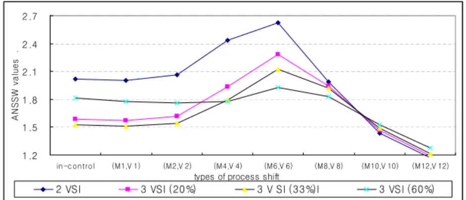
In Figure 4.5, when small or moderate shifts are occurred, two sampling intervals VSI chart shows better ANSSW performances than three sampling interval VSI chart. If the process is neccessary to use three sampling intervals VSI chart, then ANSSW can be improved when design parameters g 1 , g 2 , h are carefully selected according to the scale of process change which is interesting.
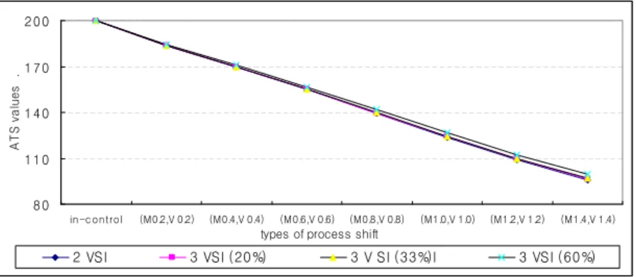
From the numerical results in Tables and Figure 4.1, ANSS and ATS values of two sampling intervals VSI chart and three sampling interval VSI chart are similar regardless the amount of shifts. Therefore, when quality engineers in industry select one of the two procedures, two sampling intervals VSI and three sampling intervals VSI chart, and their main concern are the required time to signal, ANSS and STS, then they could select either one of both under the comprehensive consideration.
However, if switching behavior, and additional efforts and costs in the process of operating VSI chart, which are mentioned as shortcoming, can not be ignored, then two sampling interval VSI chart can be still recommended.
80 110 140 170 200
in -c on trol (M0.2,V 0.2) (M0.4,V 0.4) (M0.6,V 0.6) (M0.8,V 0.8) (M1.0,V 1.0) (M1.2,V 1.2) (M1.4,V 1.4) types of process shift
ATS values .
2 VSI 3 VSI (20%) 3 V SI (33%)I 3 VSI (60%)
Figure 4.1 ATS of the two and three sampling intervals VSI charts (p =5)
50 80 110 140
in -c on trol (M0.2,V 0.2) (M0.4,V 0.4) (M0.6,V 0.6) (M0.8,V 0.8) (M1.0,V 1.0) (M1.2,V 1.2) (M1.4,V 1.4) types of process shift
ANSW values .
2 VSI 3 VSI (20%) 3 V SI (33%)I 3 VSI (60%)
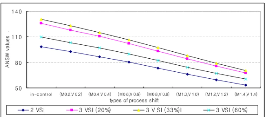
Figure 4.2 ANSW of the two and three sampling intervals VSI charts (p =5)
0.4 0.6 0.8 1.0
in -c on trol (M1,V 1) (M2,V 2) (M4,V 4) (M6,V 6) (M8,V 8) (M10,V 10) (M12,V 12) types of process shift
ASI values .
2 VSI 3 VSI (20%) 3 V SI (33%)I 3 VSI (60%)
Figure 4.3 ASI of the two and three sampling intervals VSI charts (p =5)
0.3 0.5 0.7 0.9
in -c on trol (M1,V 1) (M2,V 2) (M4,V 4) (M6,V 6) (M8,V 8) (M10,V 10) (M12,V 12) types of process shift
ASWR values .
2 VSI 3 VSI (20%) 3 V SI (33%)I 3 VSI (60%)
Figure 4.4 ASWR of the two and three sampling intervals VSI charts (p =5)
1.2 1.5 1.8 2.1 2.4 2.7
in -c on trol (M1,V 1) (M2,V 2) (M4,V 4) (M6,V 6) (M8,V 8) (M10,V 10) (M12,V 12) types of process shift
ANSSW values .