Switching performances of multivarite VSI chart for simultaneous monitoring correlation coefficients of related quality variables

Switching performances of multivarite VSI chart for simultaneous monitoring correlation coefficients of

related quality variables ^†

Duk-Joon Chang ¹

1 Department of Statistics, Changwon National University

Received 28 February 2017, revised 16 March 2017, accepted 20 March 2017

Abstract

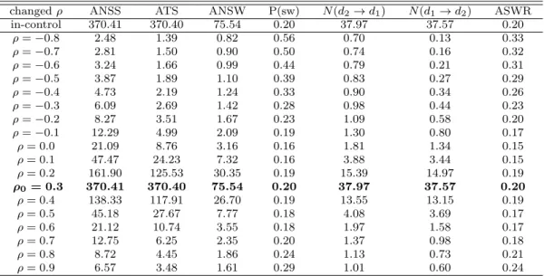
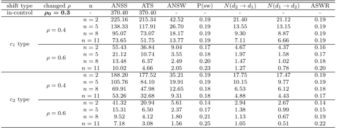
There are many researches showing that when a process change has occurred, vari- able sampling intervals (VSI) control chart is better than the fixed sampling interval (FSI) control chart in terms of reducing the required time to signal. When the process engineers use VSI control procedure, frequent switching between different sampling in- tervals can be a complicating factor. However, average number of samples to signal (ANSS), which is the amount of required samples to signal, and average time to sig- nal (ATS) do not provide any control statistics about switching performances of VSI charts. In this study, we evaluate numerical switching performances of multivariate VSI EWMA chart including average number of switches to signal (ANSW) and av- erage switching rate (ASWR). In addition, numerical study has been carried out to examine how to improve the performance of considered chart with accumulate-combine approach under several different smoothing constant and sample size. In conclusion, process engineers, who want to manage the correlation coefficients of related quality variables, are recommended to make sample size as large and smoothing constant as small as possible under permission of process conditions.

Keywords: ANSW, ATS, moment generating function, Shewhart chart, switching be- havior.

1. Introduction

In many industrial quality control, the quality of an output is usually characterized by joint levels of associated quality variables rather than a single one. And shifts in correlation coefficients of associated quality variables should be considered importantly when linear relationship among more than two quality variables largely effect the quality of product.

Especially in chemical industry, relatively small amount of change of correlation coefficients among quality variables often gives large effect on product quality.

When the statistical quality control chart indicates that the production process is currently under in-control state or stable, then no corrections or changes to process control parameters

† This research is financially supported by Changwon National University in 2017-2018.

1 Professor, Department of Statistics, Changwon National University, Changwon 51140, Korea.

E-mail: [email protected]

are needed or desired. In this case, data from the production process can be used to predict the future performance of the process or product. However if the control chart indicates that the monitored process is out-of-control state, then a rectifying action is needed to remove the reasonable cause and turn the out-of-control state into in-control state. Control chart is widely used traditional technique to show quality data from a production process for quick monitoring whether a process is in-control state or not.

The EWMA chart, first introduced by Roberts (1959), has approximately equivalent per- formances to the CUSUM chart and has a good ability when we are interested in detecting small or moderate shifts. And Hotelling (1947) originally proposed multivariate control chart.

Alt (1984) and Jackson (1985) reviewed many articles on multivariate chart.

Lowry et al. (1992) presented a MEWMA chart for mean vector of multiple quality vari- ables with accumulate-combine approach that accumulate past sample information for each paramter and then combines the separate accumulations of each process parameter into a univariate control statistic. Through simulation, they showed that the performances of MEWMA chart are better than the multivariate CUSUM charts which are proposed by Pignatiello and Runger (1990) and Crosier (1988), and stated that MEWMA procedure is easy to design and implement. We can see recent works on Multivariate quality control pro- cedures in Jeong and Cho (2012), Park and Cho (2013) and Hwang (2016). Chang (2015) compared three sampling intervals VSI procedure with two sampling intervals VSI procedure for multivariate normal process.

The change of correlation coefficients, explaining the strength of linear relationship be- tween two or more quality variables, often makes effect considerably on the quality of prod- ucts. However, it is hard to find researches up to present, monitoring correlation coeffi- cients of several related quality variable at the same time. This paper focused both on the ANSS/ATS performances and switching properties of multivarite EWMA chart with accumulate-combine approach for simultaneously monitoring every correlation coefficients of p (p ≥ 2) related multiple quality variables.

In this paper, we evaluated numerical properties of the considered multivariate chart with accumulate-combine approach to simultaneously monitor all correlation coefficients of several related quality characteristics under multivariate normal process.

2. Fixed sampling interval scheme

The traditional method of control chart is FSI chart, which selects samples with equal time interval, and the performances of proposed control charts are evaluated and compared based on FSI chart. In FSI chart, the number of samples required for the chart to signal is the run length (RL), and expected value of the RL is the ARL. Therefore, the ARL in FSI chart can be thought of as the ANSS. And the usual practice behind most statistical quality control techniques is that there are 4 or 5 observations for each variables of the production process at each sampling occasion.

Suppose that there are p (p ≥ 2) variables that explain the quality of products and

they have multivariate normal N (µ, Σ). Let the sample of size n observations taken at

any sampling time i (i = 1, 2, 3, · · · ) be represented by X _i = (X ⁰ _i1 , X ⁰ _i2 , · · · , X ⁰ _in ) ⁰ and

X _ij = (X _ij1 , X _ij2 , · · · , X _ijp ) ⁰ . In addition, suppose that the observations have independent

multivariate normal distribution N (µ, Σ).

Let θ = (µ, Σ) be the process parameters of associated quality variables, and θ ₀ = (µ

0 , Σ ₀ ) be its known value, where µ is mean vector and Σ is dispersion matrix of X. For simplicity in our numerical computation, we assume that µ

0 = 0 ⁰ and target dispersion matrix Σ 0 has values 1 for all diagonal components and 0.3 for all off-diagonal components.

To monitor the correlation coefficient ρ 12 of two quality variables X 1 and X 2 , we can con- sider a univariate control chart for ρ 12 under the condition that µ 10 , µ 20 , σ 10 and σ 20 are the known target process means and standard deviations of X 1 and X 2 . The correlation coeffi- cient of two quality variables X 1 and X 2 , ρ 12 , is estimated with r 12 =

P

n

j=1

(x

_1j

−µ

1

)(x

_2j

−µ

2

) nσ

1

σ

2

and the univariate EWMA chart for one correlation coefficient ρ ₁₂ can be formulated as Y i = (1 − λ)Y i−1 + λ

P

n

j=1

(X

ij1

−µ

10

)(X

ij2

−µ

20

)

nσ

₁₀

σ

₂₀

(i = 1, 2, · · · ) and 0 < λ ≤ 1.

This Y i can be expressed as follows

Y i = (1 − λ) ⁱ Y 0 +

i

X

k=1

λ(1 − λ) ^i−k

n

P

j=1

(X kj1 − µ 10 )(X kj2 − µ 20 )

nσ ₁₀ σ ₂₀ (2.1)

To monitor all correlation coefficients of p associated quality variables simultaneously, let ρ = (ρ ₁₂ , ρ ₁₃ , · · · , ρ _1p , ρ ₂₃ , · · · , ρ _2p , · · · , ρ _p−1,p ) ⁰ and

Y ⁰ _i = (Y _i1 , Y _i2 , · · · , Y _i,p−1 , Y _ip , · · · , Y _i,2p−3 , · · · , Y _i,s−1 , Y _i,s ).

where s = p(p − 1)/2. Then the vector of EWMA’s can be written as

Y _i =























































(1 − λ ₁ ) ⁱ Y _i10 +

i

P

k=1

λ ₁ (1 − λ ₁ ) ^i−k CR _k12 .. .

(1 − λ p−1 ) ⁱ Y i,p−1,0 +

i

P

k=1

λ p−1 (1 − λ p−1 ) ^i−k CR k1p

(1 − λ _p ) ⁱ Y _i,p,0 +

i

P

k=1

λ _p (1 − λ _p ) ^i−k CR _k23 .. .

(1 − λ 2p−3 ) ⁱ Y i,2p−3,0 +

i

P

k=1

λ 2p−3 (1 − λ 2p−3 ) ^i−k CR k2p

.. . (1 − λ s ) ⁱ Y i,s,0 +

i

P

k=1

λ s (1 − λ s ) ^i−k CR k,p−1,p























































, (2.2)

where 0 < λ a ≤ 1(a = 1, 2, · · · , s) and CR kmu =

P

n

j=1

(X

kjm

−µ

m0

)(X

kju

−µ

u0

)

nσ

_m0

σ

_u0

− ρ mu0 (m 6= u).

Multivariate EWMA chart based on the vector (2.2) can be expressed as

Y _i =

i

X

k=1

Λ(I − Λ) ^i−k CR _k + (I − Λ) ⁱ Y ₀ (2.3)

where

CR ⁰ _k = (CR _k12 , CR _k13 , · · · , CR _k1p , CR _k23 , · · · , CR _k2p , · · · , CR _k,p−1,p ), smoothing matrix Λ = diag(λ ₁ , λ ₂ , · · · , λ _s ) and 0 < λ _j ≤ 1 (j = 1, 2, · · · , s).

For simplicity in our numerical computation, we set all diagonal elements of the smoothing matrix Λ to be equal. Under this assumption that λ ₁ = λ ₂ = · · · = λ _s = λ, the multivariate EWMA vector in (2.3) can be written as

Y _i = (1 − λ)Y _i−1 + λCR _i

=

i

X

k=1

λ(1 − λ) ^i−k CR _k + (1 − λ) ⁱ Y ₀ .

This multivariate EWMA chart for ρ = (ρ ₁₂ , ρ ₁₃ , · · · , ρ _1p , ρ ₂₃ , · · · , ρ _2p , · · · , ρ _p−1,p ) ⁰ signals whenever

T _i ² = Y ⁰ _i Σ _Y

_i

Y _i > h.

The upper control limit (UCL) h is determined to satisfy a specified ANSS by simulation.

And the variance-covariance matrix Σ _Y

i

with dimension s × s is as follows Σ Y

_i

=

( λ[1 − (1 − λ) ²ⁱ ] 2 − λ

)

· Σ CR

and

Σ CR =











V ar(CR i12 ) Cov(CR i12 , CR i13 ) · · · Cov(CR i12 , CR t,p−1,p ) V ar(CR i13 ) · · · Cov(CR i13 , CR i,p−1,p )

. . . .. .

Sym V ar(CR ip−1,p )









 ,

where

V ar(CR ipq ) = 1 + ρ ² _pq0 n

Cov(CR _ipq , CR _ipr ) = ρ qr0 + ρ pq0 ρ pr0

n

Cov(CR _ipq , CR _irw ) = ρ _pr0 ρ _qw0 + ρ _pw0 ρ _qr0 n

and the subscripts p, q, r and w are different each other. The components in Σ CR are obtained using the moment generating function of multivariate normal distribution N (µ, Σ).

3. Variable sampling intervals scheme

The problem of determining sampling plans with VSI scheme was first investigated by

Arnold (1970). The basic idea of VSI control scheme is that if there are some signs of

process change then the sampling interval is expected to be short and if there is no sign of process change then the sampling interval is expected to be long. If the sign of a process change is over the UCL, then both the VSI and FSI charts give signal.

In FSI scheme, the sampling interval between samples is fixed. But for a VSI control scheme, the sampling time intervals are random and depends on T ₁ ² , T ₂ ² , · · · , T _i ² . Therefore in VSI scheme, the time to signal is not the product of RL and a fixed value. Thus for evaluating the performances of a VSI chart, both the time to signal (TS) and the number of samples to signal (NSS) need to be considered. Following the definitions of Reynolds et al.(1988), the expected value of the NSS is ANSS and the expected value of the TS is ATS.

The properties of VSI chart were investigated by Reynolds et al. (1990), Amin and Miller (1993). According to Reynolds and Arnold (1989) and Reynolds (1989), the VSI chart is better than FSI chart in terms of ATS and ANSS. They also showed that the two sampling intervals VSI chart is optimal for larger gap between two sampling intervals for one- and two-sided Shewhart chart.

The weakness of VSI scheme is that when an engineer applies the scheme, frequent switch- ing sampling intervals requires more efforts and costs than FSI scheme.

Amin and Hemasinha (1993), Shamma et al. (1991) and Amin and Letsinger (1991) studied the switching property of VSI charts.

In VSI charts, frequent switching is a complicating factor. Hence the small number of switching is desirable for both in-control and out-of-control states. Since ANSS and ATS do not directly provide any information on how frequently switches are made, VSI procedures require new quantities measuring the switching frequency.

Up to the present, many articles investigated the efficiency of a VSI chart in terms of ATS and ANSS when the process has changed.

Amin and Letsinger (1991) gave some idea to combine VSI charts, and they also inves- tigated switching property and runs rules with different sampling intervals. They showed that the ANSW of the CUSUM and EWMA charts are much smaller than the Shewhart chart’s. Bai and Lee (2002) used Markov chain approach to express the ATS and ANSW and suggested three switching rules of the ¯ X control charts.

For the VSI EWMA chart based on Y _i in (2.2), let the sampling interval be;

d ₁ for T _i ² ∈ (g, h], d ₂ for T _i ² ∈ (0, g], where g ≤ h and d ₁ < d ₂ .

If the chart statistic T _i ² is over the UCL h, then both FSI and VSI charts give signal.

Since it is difficult to obtain the distribution of chart statistic Y _i , the process parameters h, g can be obtained to satisfy a specified ATS and ANSS. The numerical performances and switching properties of this chart is evaluated through simulation work for both in-control and shifted.

In VSI chart, the sampling intervals are random, and samples are taken irregular time intervals. Therefore, It is necessary to consider a quantity which measures the frequency of switches between different sampling intervals in VSI structure.

To estimate the efficiency of applied VSI procedures, it is necessary to obtain the average

number of switches (ANSW) made from the beginning of the process until the procedure

gives signals. The ANSW can be obtained by using Wald’s identity as follows AN SW = (AN SS − 1) · P (switch).

And, the switch probability is measured as

P (switch) = P (d 1 ) · P (d 2 |d 1 ) + P (d 2 ) · P (d 1 |d 2 )

where P (d i ) is the probability of d i , and P (d i |d j ) is the probability of d i conditional on the previous sampling interval d j (d i 6= d j ). To quantify the amount of switching performance of a VSI chart, the average switching rate (ASWR) is defined by

ASW R = AN SW/AN SS.

Like ANSW, a low ASWR is usually desirable in industry, but the ASWR close to zero is not realistic. The N (d2 → d1) and N (d1 → d2) in Tables indicate the numbers of switches, that the sampling interval changes from d ₁ to d ₂ or vice versa, to signal when the process has changed.

4. Switching performances and concluding remarks

In this paper, we considered multivariate chart with accumulate-combine approach for monitoring every correlation coefficients of related quality variables under multivariate nor- mal process. Since it is difficult to obtain the distribution of sample statistic Y _i in (2.2), the design parameters h, g and numerical performances including switching behaviors of the considered chart can be evaluated by simulation with 10,000 iterations under the parameters of the process is on-target or changed.

In our simulation, the ANSS and ATS under in-control state was set to be 370.4 and the sample size n to be 5 for p = 3 and p = 4. And we set d = 1 in FSI chart and d 1 = 0.1 and d 2 = 1.9 in VSI chart. The types of process changes under out-of-control state is stated as follows :

(c1) ρ 12 and ρ 21 have changed

(c2) all ρ 1j and ρ j1 (j = 2, · · · , p) have changed

After that the design parameters h and g of the considered multivariate EWMA chart based on Y _i in (2.2) has been determined, the ANSS, ATS and switching performances including ANSW under (c1) and (c2) were obtained with 10,000 iterations.

The numerical results of the considered multivariate VSI EWMA chart are presented in Table 4.1 ∼ Table 4.4. Performances and switching properties of the chart for process in- control and out-of-control states are presented in for p = 3 and 4. Table 4.1 and Table 4.2 show that when the size of the shift is increasing, ANSS, ATS, ANSW have a tendency to decrease but P (switch) and ASWR show the tendency to increase. And we also found that regardless of the size of shift, VSI scheme is superior to FSI in terms of ANSS and ATS.

When the process change has occurred, the required time to signal can be thought of as

ANSS in FSI scheme and ATS in VSI scheme. And now, all the Tables show that ATS is

smaller than ANSS when the process has changed.

Table 4.1 Numerical results for the considered VSI chart (p=3, λ = 0. 1, n=5)

changed ρ ANSS ATS ANSW P(sw) N (d 2 → d 1 ) N (d 1 → d 2 ) ASWR

in-control 370.41 370.40 75.54 0.20 37.97 37.57 0.20

ρ = −0.8 2.48 1.39 0.82 0.56 0.70 0.13 0.33

ρ = −0.7 2.81 1.50 0.90 0.50 0.74 0.16 0.32

ρ = −0.6 3.24 1.66 0.99 0.44 0.79 0.21 0.31

ρ = −0.5 3.87 1.89 1.10 0.39 0.83 0.27 0.29

ρ = −0.4 4.73 2.19 1.24 0.33 0.90 0.34 0.26

ρ = −0.3 6.09 2.69 1.42 0.28 0.98 0.44 0.23

ρ = −0.2 8.27 3.51 1.67 0.23 1.09 0.58 0.20

ρ = −0.1 12.29 4.99 2.09 0.19 1.30 0.80 0.17

ρ = 0.0 21.09 8.76 3.16 0.16 1.81 1.34 0.15

ρ = 0.1 47.47 24.23 7.32 0.16 3.88 3.44 0.15

ρ = 0.2 161.90 125.53 30.35 0.19 15.39 14.97 0.19

ρ 0 = 0.3 370.41 370.40 75.54 0.20 37.97 37.57 0.20

ρ = 0.4 138.33 117.91 26.70 0.19 13.55 13.15 0.19

ρ = 0.5 45.18 27.67 7.77 0.18 4.08 3.69 0.17

ρ = 0.6 21.12 10.74 3.55 0.18 1.97 1.58 0.17

ρ = 0.7 12.75 6.25 2.35 0.20 1.37 0.98 0.18

ρ = 0.8 8.72 4.45 1.86 0.24 1.13 0.73 0.21

ρ = 0.9 6.57 3.48 1.61 0.29 1.01 0.60 0.24

Table 4.2 Numerical results for the considered VSI chart (p=4, λ = 0. 1, n=5)

changed ρ ANSS ATS ANSW P(sw) N (d 2 → d 1 ) N (d 1 → d 2 ) ASWR

in-control 370.40 370.40 74.81 0.20 37.60 37.22 0.20

ρ = −0.7 3.08 1.74 1.01 0.49 0.76 0.25 0.33

ρ = −0.6 3.58 1.95 1.11 0.43 0.80 0.31 0.31

ρ = −0.5 4.28 2.21 1.22 0.37 0.85 0.36 0.28

ρ = −0.4 5.25 2.58 1.36 0.32 0.92 0.44 0.26

ρ = −0.3 6.72 3.16 1.54 0.27 1.00 0.54 0.23

ρ = −0.2 9.11 4.10 1.84 0.23 1.15 0.69 0.20

ρ = −0.1 13.57 5.88 2.33 0.19 1.38 0.95 0.17

ρ = 0.0 23.83 10.44 3.61 0.16 2.02 1.59 0.15

ρ = 0.1 55.08 29.88 8.81 0.16 4.61 4.20 0.16

ρ = 0.2 177.48 143.70 33.79 0.19 17.09 16.70 0.19

ρ 0 = 0.3 370.40 370.40 74.81 0.20 37.60 37.22 0.20

ρ = 0.4 172.37 148.09 33.25 0.19 16.82 16.43 0.19

ρ = 0.5 54.60 33.36 9.36 0.18 4.88 4.49 0.17

ρ = 0.6 24.90 12.45 4.05 0.17 2.22 1.83 0.16

ρ = 0.7 14.55 7.16 2.62 0.19 1.51 1.12 0.18

ρ = 0.8 9.89 5.08 2.06 0.23 1.22 0.83 0.21

ρ = 0.9 7.28 3.94 1.75 0.28 1.07 0.68 0.24

In Table 4.3, for each shifted type of process change c1 and c2, when the target value is

changed from ρ ₀ = 0.3 to 0.4 and 0.6, the performance and switching property are calculated

for different sample size n. Table 4.3 shows that as the sample size n is increasing form 2 to 5,

8, and 11, the performance and switching property of considered EWMA chart is improved

rapidly. Therefore, process engineers, who want to manage the correlation coefficients of

related quality variables, are recommended to make sample size n as large as possible under

permission of process conditions.

Table 4.3 Numerical results of different n for the considered VSI chart (p = 3, λ = 0.1) shift type changed ρ n ANSS ATS ANSW P(sw) N (d

2

→ d

₁

) N (d

1

→ d

₂

) ASWR

in-control ρ

0

= 0.3 - 370.40 370.40 - - - - -

c

1

type

ρ = 0.4

n = 2 225.16 215.34 42.52 0.19 21.40 21.12 0.19

n = 5 138.33 117.91 26.70 0.19 13.55 13.15 0.19

n = 8 95.07 73.07 18.17 0.19 9.30 8.87 0.19

n = 11 73.65 51.75 13.77 0.19 7.11 6.66 0.19

ρ = 0.6

n = 2 55.43 36.84 9.04 0.17 4.67 4.37 0.16

n = 5 21.12 10.74 3.55 0.18 1.97 1.58 0.17

n = 8 13.48 6.37 2.49 0.20 1.47 1.02 0.18

n = 11 10.02 4.66 2.05 0.23 1.27 0.78 0.20

c

2

type

ρ = 0.4

n = 2 188.20 177.52 35.21 0.19 17.75 17.47 0.19

n = 5 105.76 84.10 19.91 0.19 10.15 9.77 0.19

n = 8 69.91 47.98 12.65 0.18 6.53 6.12 0.18

n = 11 53.26 32.68 9.31 0.18 4.88 4.43 0.17

ρ = 0.6

n = 2 41.32 20.94 5.61 0.14 2.94 2.67 0.14

n = 5 15.31 6.50 2.37 0.17 1.38 0.99 0.15

n = 8 9.52 4.12 1.80 0.21 1.13 0.67 0.19

n = 11 7.18 3.08 1.56 0.25 1.05 0.51 0.22

Table 4.4 shows the performances according to the change of size of the smoothing constant λ. In Table 4.4, we can find that the smaller the smoothing constant λ ⁰ _i s are, the better the detecting any sizes of changes is in terms of ANSS and ATS. And we also found that smaller values of the parameter λ will reduce the switching performances ANSW, P (sw), N (d 1 → d 2 ) and N (d 2 → d 1 ). Usually, the optimal selection of λ in EWMA chart depends on the size of the shift to detect quickly. And we also recommend that small value of λ is preferred for detecting small or moderate changes vice versa for various p.

Table 4.4 Numerical results of different λ for the considered VSI chart (p=3, n=5)

shift type changed ρ λ ANSS ATS ANSW P(sw) N (d

2

→ d

1

) N (d

1

→ d

2

) ASWR

in-control ρ

0

= 0.3 - 370.4 370.4 - - - - -

c

1

type

ρ = 0.4

λ = 0.1 138.33 117.91 26.70 0.19 13.55 13.15 0.19

λ = 0.2 186.08 173.04 50.13 0.27 25.24 24.89 0.27

λ = 0.3 216.44 208.40 70.71 0.33 35.50 35.21 0.33

λ = 0.4 236.66 232.11 88.13 0.37 44.17 43.96 0.37

λ = 0.5 253.52 251.51 104.07 0.41 52.11 51.96 0.41

λ = 0.6 266.71 266.62 117.90 0.44 59.00 58.90 0.44

λ = 0.7 276.97 278.27 129.33 0.47 64.69 64.64 0.47

λ = 0.8 283.47 285.92 137.52 0.49 68.77 68.75 0.49

λ = 0.9 287.91 290.97 142.88 0.50 71.44 71.44 0.50

λ = 1.0 293.47 297.09 146.59 0.50 73.29 73.30 0.50

ρ = 0.6

λ = 0.1 21.12 10.74 3.55 0.18 1.97 1.58 0.17

λ = 0.2 32.07 17.96 6.69 0.22 3.55 3.14 0.21

λ = 0.3 45.15 29.72 12.04 0.27 6.21 5.83 0.27

λ = 0.4 59.59 44.32 19.10 0.33 9.71 9.39 0.32

λ = 0.5 73.09 59.43 26.94 0.37 13.61 13.34 0.37

λ = 0.6 86.73 75.20 35.52 0.41 17.87 17.65 0.41

λ = 0.7 99.72 90.64 44.22 0.45 22.19 22.03 0.44

λ = 0.8 109.98 103.67 51.69 0.47 25.90 25.79 0.47

λ = 0.9 118.69 114.99 58.04 0.49 29.05 28.99 0.49

λ = 1.0 126.12 124.75 63.04 0.50 31.53 31.51 0.50

c

2

type

ρ = 0.4

λ = 0.1 105.76 84.10 19.91 0.19 10.15 9.77 0.19

λ = 0.2 146.56 132.63 38.68 0.27 19.51 19.17 0.26

λ = 0.3 173.22 165.49 55.77 0.32 28.02 27.75 0.32

λ = 0.4 193.88 190.59 71.45 0.37 35.83 35.62 0.37

λ = 0.5 208.88 208.97 85.09 0.41 42.62 42.47 0.41

λ = 0.6 223.41 225.90 98.16 0.44 49.12 49.04 0.44

λ = 0.7 234.72 239.06 109.05 0.47 54.55 54.50 0.46

λ = 0.8 244.50 250.11 118.28 0.49 59.15 59.13 0.48

λ = 0.9 252.10 258.81 124.85 0.50 62.42 62.43 0.50

λ = 1.0 255.49 262.69 127.53 0.50 63.75 63.78 0.50

ρ = 0.6

λ = 0.1 15.31 6.50 2.37 0.17 1.38 0.99 0.15

λ = 0.2 23.23 9.37 3.72 0.17 2.07 1.65 0.16

λ = 0.3 33.13 16.13 7.09 0.22 3.74 3.34 0.21

λ = 0.4 44.25 26.40 12.33 0.29 6.34 5.98 0.28

λ = 0.5 55.17 38.46 18.67 0.35 9.49 9.18 0.34

λ = 0.6 65.82 51.30 25.51 0.39 12.88 12.63 0.39

λ = 0.7 75.24 63.72 32.29 0.44 16.24 16.06 0.43

λ = 0.8 83.81 75.50 38.69 0.47 19.41 19.28 0.46

λ = 0.9 91.98 86.74 44.65 0.49 22.36 22.29 0.49

λ = 1.0 99.28 96.91 49.69 0.51 24.86 24.84 0.50

References

Alt, F. B. (1984). Multivariate control charts. In Encyclopedia of Statistical Sciences, edited by S. Kotz and M. L. Johnson, Wiley, New York.

Amin, R. W. and Hemasinha, R. (1993). The switching behavior of ¯ X charts with variable sampling intervals.

Communications in Statistics-Theory and Methods, 22, 2081-2102.

Amin, R. W. and Letsinger, W. C. (1991). Improved switching rules in control procedures using variable sampling intervals. Communications in Statistics-Simulation and Computation, 20, 205-230.

Amin, R. W. and Miller, R. W. (1993). A robustness study of ¯ X charts with variable sampling intervals.

Journal of Quality Technology, 25, 36-44.

Arnold, J. C. (1970). A Markovian sampling policy applied to quality monitoring of streams. Biometrics, 26, 739-747.

Bai, D. S. and Lee, K. T. (2002). Variable sampling interval ¯ X control charts with an improved switching rule. International Journal of Production Economiccs, 76, 189-199.

Chang, D. J. (2015). Comparison of two sampling intervals and three sampling intervals VSI charts for monitoring both means and variances. Journal of the Korean Data & Information Science Society, 26, 997-1006.

Crosier, R. B. (1988). Multivariate generalization of cumulative sum quality-control scheme. Technometrics, 30, 291-303.

Hotelling, H. (1947). Multivariate quality control. Techniques of Statistical Analysis, McGraw-Hill, New York, 111-184.

Hwang, C. (2016). Multioutput LS-SVR based residual MCUSUM control chart for autocorrelated process.

Journal of the Korean Data & Information Science Society, 27, 523-530.

Jackson, J. E. (1985). Multivariate quality control. Communications in Statistics-Theory and Method , 14, 2657-2688.

Jeong, J. I. and Cho, G. Y. (2012). Multivariate Shewhart control charts for monitoring the variance- covariance matrix. Journal of the Korean Data & Information Science Society, 23, 617-628.

Lowry, C. A., Woodall, W. H., Champ, C. W. and Rigdon, S. E. (1992). A multivariate exponentially weighted moving average control charts. Technometrics, 34, 46-53.

Park, J. S. and Cho, G. Y. (2013). Parameter estimation in a readjustment procedures in the multivariate integrated process control. Journal of the Korean Data & Information Science Society, 24, 1275-1283.

Pignatiello, J. J. and Runger, G. C. (1990). Comparisons of multivariate CUSUM charts. Journal of Quality Technology, 22, 173-186.

Reynolds, Jr, M. R. (1989). Optimal variable sampling interval control charts with variable sampling inter- vals. Sequential Analysis, 8, 361-379.

Reynolds, Jr, M. R., Amin, R. W. and Arnold, J. C. (1990). CUSUM charts with variable sampling intervals.

Technometrics, 32, 371-384.

Reynolds, Jr, M. R., Amin, R. W., Arnold, J. C. and Nachalas, J. A. (1988). ¯ X - charts with variable sampling intervals. Technometrics, 30, 181-192.

Reynolds, Jr, M. R. and Arnold, J. C. (1989). Optimal one-sided Shewhart control charts with variable sampling intervals between samples. Sequential Analysis, 8, 51-77.

Roberts, S. W. (1959). Control chart tests based on geometric moving averages. Technometrics, 1, 239-250.

Shamma, S. E., Amin, R. W. and Shamma, A. K. (1991). A double exponentially weighted moving aver-

age control procedure with variable sampling intervals. Communications in Statistics-Simulation and

Computation, 20, 511-528.