The relation between the catch of yellowfin tuna (Thunnus albacares) and marine environment in the northwestern Indian Ocean
Kuo-Wei Lan1, Ming-An Lee1 and Tom Nishida2
1Department of Environmental Biology and Fisheries Science, National Taiwan Ocean University, 2 Pei-Ning Road, Keelung, Taiwan 20224 R.O.C
2National Research Institute of Far Seas Fisheries, Fisheries Research Agency, 5-7-1, Orido,Shimizu-Ward, Shizuoka-City, Shizuoka, Japan 4248633
Present email address: [email protected]
Introduction
Yellow-fin tuna is one of the major target fishes of the Taiwanese commercial tuna longline (LL) fishery in the northwestern Indian Ocean. Previous research indicated that the YFT's distribution is mostly concentrated in the Arabian Sea, western tropical waters, and regions around Madagascar (FAO, 1994). Although the Arabian Sea is an important area for Taiwanese LL fishery to exclusively target the YFT in the northwestern Indian Ocean, meso-scale research evaluating the impacts of environmental and oceanographic variables on the fishery is not yet well understood in the Arabian Sea despite the long exploitation history of the YFT. The biophysical environment plays important roles in controlling the distribution and abundance of tuna (Lee et al., 1999). In this study, we collected the longliners data caught by Taiwan longline fleet and environment variables from multiple satellite data and model-simulated sub-surface data. Remote sensing techniques have great potential to support global fisheries management and the exploitation of pelagic fishes (Zagaglia et al., 2004). In a comprehensive study of the environmental preferences of the YFT and consider the cause of the abnormally high catch in the Arabian Sea.
Data and Method
The catch and effort data of the Taiwanese LL fishery in the Arabian Sea at 10°~30°N and 40°~80°E were provided by the Oversea Fisheries Development Council (OFDC) of Taiwan. We used five satellite-derived and model-simulated data in this study: (1) chlorophyll-a concentration (Chl-a); (2) sea surface temperature (SST); (3) Precipitation (Pr); (4) wind speed (WS) and (5) model simulated sea temperatures (ST) and salinity (SS) at depths of 5~459 m. The fishery data and environmental data were geographically to monthly means on the 5°x 5° spatial grid during the period of 1998 to 2004 for analysis.
The CPUE was used as a relative abundance index of the YFT. It was calculated as the number of individuals captured by 1000 hooks (fish/1000 hooks) on a 5°x 5° spatial resolution grid, and values were integrated into monthly averages. The CPUE in relation with environmental factors were predicted by the principal component analysis (PCA).
Results and Discussion
The catch per unit effort (CPUE) was calculated as the number of fish caught by 1000 hooks in 5°×5° degree square grid and showed that the fishing season was from February to July (Figure.1), the averaged CPUE was 13.21 (inds/1000 hooks) and a high CPUE occurred in April and May. In 1998 to 2004, the yearly mean catch of the YFT was 5453 metric tons (mt), but in 2005 the total catch was 6-fold more than other years and increased to 34239 mt.
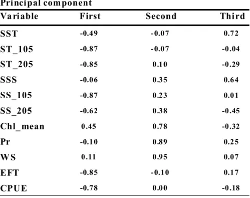
The percentage variance and eigenvalue of each principal component showed that the three principal components had eigenvalues of > 1 (Table.1), which accounted for 77.31% of the cumulative variance. Factor loadings of the first three components of the PCA of 11 variables are listed in Table 2. The result of PCA shows monthly variations in YFT CPUE values were significantly related to the sub-surface temperature and sub-surface salinity. During the high CPUE period (in April and May) were the warmest months of the year, the sub-surface temperature and Salinity between 105~205 m was 16.08~24.28°C and 35.74~36.19 psu. Stretta (1991) indicated that in the tropics, most YFTs preferred warm water with a narrow temperature range of 22~29°C, particularly above 25°C. The Taiwanese LL fishery targeting YFT has an operating depth of 50~120 m in the Indian Ocean (Lee, Nishida & Mohri, 2005), where temperatures generally exceed 20 °C, and the YFT is abundant. After July, a drop in the temperature to below the preferred temperature range for the YFT is probably the reason that CPUE subsequently decreased from July to December.
The results also shows the reasons cause the high catch and high CPUE throughout 2005 whole year because of the increase of the vertical sea temperature and salinity in the northwestern Indian Ocean (Figure.2).
References
FAO Fisheries Department, 1994. World review of highly migratory species and straddling stocks.
FAO Fish. Tech. Pap. 337, 70 pp.
Lee, P.F., Chen, I.C., Tseng, W.N., 1999. Distribution patterns of three dominant tuna species in the Indian Ocean. 19th Intern. ERSI Users Conf., San Diego, CA.
Lee, Y.C., Nishida, T., Mohri, M., 2005. Separation of the Taiwanese regular and deep tuna longliners in the Indian Ocean using bigeye tuna catch ratios. Fish. Sci. 71, 1256-1263.
Stretta, J.M. 1991. Forecasting models for tuna fishery with aeroespatial remote sensing. Int. J.
Remote Sens. 12(4), 771-779.
Zagaglia, C. R., Lorenzzetti, J. A., Stech, J. L., 2004. Remote sensing data and longline catches of yellowfin tuna (Thunnus albacares) in the equatorial Atlantic. Remote Sens. Environ., 93, 267-281.
Table 1. Eigenvalues and the variance cumulative percentage (Prin1~4) for the principal component analysis
Principle componrnt Eigenvalue variance(%) Cumulative EVL Cumulative(%)
PRIN1 4.41 40.05 4.41 40.05
PRIN2 2.66 24.15 7.06 64.20
PRIN3 1.44 13.11 8.50 77.31
PRIN4 0.94 8.53 9.44 85.84
Table 2. Results of the principal component analysis (Prin1~3) for environmental factors with yellowfin tuna catch per unit effort (CPUE)
Principal component
Va riable First Second Third
SST -0.49 -0.07 0.72
ST_105 -0.87 -0.07 -0.04
ST_205 -0.85 0.10 -0.29
SSS -0.06 0.35 0.64
SS_105 -0.87 0.23 0.01
SS_205 -0.62 0.38 -0.45
Chl_ mean 0.45 0.78 -0.32
Pr -0.10 0.89 0.25
W S 0.11 0.95 0.07
EFT -0.85 -0.10 0.17
CPUE -0.78 0.00 -0.18
0 2000 4000 6000 8000 10000 12000
1998 1999 2000 2001 2002 2003 2004 2005 2006
Catch (ton)
0 5 10 15 20 25 30 35 40 45 50 55
CPUE
Catch CPUE
Figure.1 Annual trends of Taiwanese longline fishery catch per unit effort (black line) and catch (gray chart) from 1998 to 2006.
15.50 15.70 15.90 16.10 16.30 16.50 16.70 16.90 17.10 17.30 17.50
1998 1999 2000 2001 2002 2003 2004 2005
35.70 35.72 35.74 35.76 35.78 35.80 35.82 35.84 35.86 35.88
ST_205 SS_205
Figure.2 Temporal variability in sea temperature and sea salinity at 205 m from 1998 to 2005.