Flow Patterns in a Spherical Vessel with Double-Stage Paddle Impeller

2단 패들 임펠러를 갖춘 구형교반조에서의 유동상태 Flow Patterns in a Spherical Vessel with

Double-Stage Paddle Impeller

이영세^*, 이준만^**

Young-Sei Lee^*, Joon-Man Lee^**

<Abstract>

A numerical algorithm for three-dimension laminar flow in an agitated vessel was established by using the spherical coordinates. Flow pattern for the double-stage paddle impeller was not dependent upon the distance of among the impeller in the agitated vessels. The numerical simulation of the flow pattern in spherical and cylindrical agitated vessel agree well with the visualization results.

Keywords : Spherical agitated vessel, Spherical coordinates, Flow pattern, Duble-stage paddle impeller, Numerical simulation

* 정회원, 교신저자 상주대학교 응용화학공학부, 교수, 工博 E-mail: [email protected])

** 정회원, 계명대학교 화학공학과 강사, 工博

* Corresponding Author, Prof., School of Applied Chemical Engineering, Sangju National University.

** Ph.D., Chemical Engineering, Keimyung University.

1. 서 론

2단 패들 임펠러를 준비한 구형교반조내의 유 동상태를 수치적으로 해석하는 경우 임펠러 및 축 부분의 경계조건은 원통좌표계에서 하지 않 으면 정확하게 표현할 수 없다. 또, 교반조 벽 부분의 경계조건은 구좌표계로 하지 않으면 정 확하게 표현할 수 없다. 따라서 교반조 벽부분 의 경계조건을 의사적인 구로 하는 것으로 구 형 교반조의 수치해석을 행했다. 그러나 어디까 지나 의사적인 것이고, 정확히 구형조를 표현할 수 있는 것은 없다.

본 연구에서는 임펠러 및 축 부분은 원통좌표 계로 교반조 벽부분은 구형좌표계로 각각 정확 한 경계조건을 주어 이 양좌표계를 교반조내에

서 접합하는 것으로 구형교반조내의 유동상태 의 수치해석을 하였다.

2. 수치해석 2.1 기초방정식

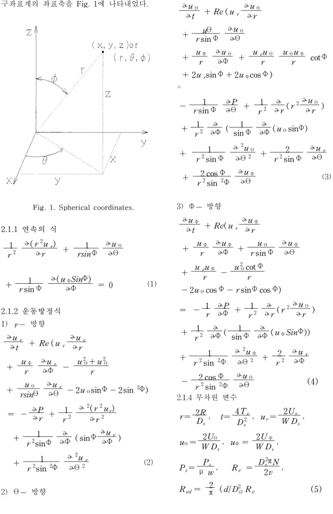
해석에 이용한 기초방정식은 원통좌표계 및 구좌표계에서의 비압축성유체의 질량보존법칙 을 나타내는 연속의 식 및 3방향의 Navior-Stokes 운동방정식을 이용하였다. 교반조내 유동상태를 수치해석하는 경우 회전좌표계에서 해석을 하 는것이 간단하기 때문에 회전구좌표계( r, θ, Φ)를 이용하였다. 해석에서 계산의 간략화를 위해 중력항을 무시하고 교반조 반경(D/2)으로 변수를 무차원화 하였다. 본 해석에서 사용한

구좌표계의 좌표축을 Fig. 1에 나타내었다.

Fig. 1. Spherical coordinates.

2.1.1 연속의 식 1

r²

ɚ(r²u_r)

ɚr + 1

rsin Φ ɚu^θ

ɚθ

+ 1

r sin Φ

ɚ(u^ΦSinΦ)

ɚΦ = 0 (1)

2.1.2 운동방정식 1) r - 방향

ɚu r

ɚt + Re ( u_r ɚur

ɚr + uΦ

r

ɚur

ɚΦ - u²θ+u²θ

r + uθ

rsinθ ɚu_r

ɚθ - 2uθsinΦ - 2 sin ²Φ) = - ɚP

ɚr + 1 r²

ɚ ²(r ²u_r) ɚr ² + 1

r²sinΦ ɚ

ɚΦ ( sinΦ ɚu_r ɚΦ )

+ 1

r²sin ²Φ

ɚ²u _r

ɚθ ² (2)

2) θ- 방향

ɚuθ

ɚt + Re ( u_r ɚuθ

ɚr

+ uθ

r sin Φ ɚuθ

ɚθ + uΦ

r

ɚuθ

ɚΦ + u _ruθ

r

uθuΦ

r cotΦ

+ 2u_rsin Φ + 2uΦcos Φ )

=

- 1

r sin Φ

ɚPɚθ + 1 r²

ɚ ɚr (r²

ɚuθ

ɚr )

+ 1

r² ɚ

ɚΦ ( 1 sin Φ

ɚ

ɚΦ ( u^θsinΦ)

+ 1

r²sin Φ

ɚ ²uθ

ɚθ² + 2

r²sin Φ ɚu_r

ɚθ + 2 cos Φ

r²sin ²Φ ɚuΦ

ɚθ (3)

3) Φ- 방향 ɚuΦ

ɚt + Re( u _r ɚuΦ

ɚr + uΦ

r

ɚu^Φ

ɚΦ + uθ

r sin Φ ɚu^Φ

ɚθ + u_ruΦ

r - u²θcot Φ r

- 2uθcos Φ - r sinΦ cos Φ)

= - 1 r

ɚΦ +ɚP 1 r²

ɚ

ɚr (r² ɚu^θ ɚr )

+ 1

r² ɚ ɚΦ ( 1

sin Φ ɚ

ɚΦ ( u^ΦSinΦ))

+ 1

r²sin ²Φ

ɚ²uΦ

ɚθ ² + 2 r²

ɚu _r ɚΦ - 2 cos Φ

r²sin ²Φ ɚu^θ

ɚθ ( 4) 2.1.4 무차원 변수

r= 2R

D_s , t= 4T_v

D_s² , ur= 2U_r W D_s , uθ= 2Uθ

W D_s , u^Φ = 2UΦ

W D_s , P_s= P_s

μ w , R_e = D_s²πN 2v , R_ed = 2

π ( d/D^2s)R_e ( 5)

위에 나타낸 회전좌표계의 기초방정식은 외 견상 정지좌표계의 식에 증가하는 형으로 나타 나고, 그 외 다른 항 및 다른 식은 양좌표계에 서 완전히 같은 형으로 나타난다. 해석은 이들 의 기초식을 유한차분법에 의해서 이산화하고 SOLA법을 이용하였다.

계산 종료 후 다음에 나타낸 식 (6)에 따라서 속도변환을 행하면 정지좌표계에서의 속도분포 를 얻을 수 있다.

u _r= u_r'

uθ= uθ' + r sin Φ

u Φ= uΦ' (6)

2.2 경계 조건 및 mesh 분할

2단 패들 임펠러에 관한 구형조에서의 해석영 역을 Fig. 2에 나타내었다.

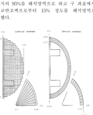
그림에서 나타난 바와 같이 원통좌표에서는 임펠러를 포함한 조 중앙에서부터 교반조벽까 지의 95%를 해석영역으로 하고 구 좌표에서는 교반조벽으로부터 15% 정도를 해석영역으로 했다.

Fig. 2. Analysed region for spherical vessel.

면은 대상으로 하는 paddle 임펠러의 날개매수 가 n_P일때 원 r-θ의 1/ n _P을 해석영역으로 했다. 또 상하 패들 임펠러의 교차각도가 0이 고, 교반조 중앙에서의 거리가 각각 같은 배치 의 2단 임펠러를 대상으로 했다. 각각의 좌표계 에서의 경계조건은 다음 식과 같이 된다.

Cylindrical coordinate

v_r = 0, vθ = 0, v_z = 0 (at shaft) vθ = 0 (at impeller)

Spherical coordinate

u_r= 0, uθ = 0, uΦ = 0 (at shaft) uθ= -r sin Φ, u_r = 0, uΦ = 0 (at impeller) (7)

또 원통좌표에서의 교반조 벽면의 경계, 및 구좌표에서의 교반조 중앙 측 경계의 초기속도 성분은 다른 방향의 좌표계에서의 속도장으로 부터 내삽에 의해 구했다. 압력은 양좌표계 모 두 축 부분에 임의로 하나의 mesh만 0으로 했 다.

2.3 수치해석의 수순

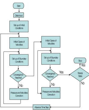
Fig. 3에 수치해석의 플로 챠트를 나타내었다.

속도장 0의 초기상태로부터 계산을 시작, 원통 좌표에서 초기속도장을 결정한다. 여기서 교반 조 벽면 측 경계의 속도 성분은 time step으로 수속한 구좌표에서의 속도성분을 이용하여 평 가한다. 그 후 time step 내에서 속도장이 연속 의 식을 만족시키게 압력 및 속도장을 보정한 다는 반복계산을 행한다. 전 mesh에 대해서 수 속을 완료한 후 구좌표에서 초기속도장을 결정 한다. 여기서 교반조 중앙 측 경계의 속도성분 은 이 time step에서 수속한 원통좌표에서의 속 도성분을 이용하여 평가한다.

그 후 원통좌표와 같은 모양으로 그 time step 내에서 속도장이 연속의 식을 만족시키게 압력 및 속도장을 보정하는 반복계산을 행한다. 전 mesh에 대해서 수속을 완료한 후 time step을 하나 진행, 양좌표에서의 속도성분이 정상상태 에 도달할 때까지 비정상적으로 계산을 수행했 다. 정상상태의 판정은 전회와 이번의 time step 간의 속도차가 양좌표의 전 mesh에 있어 서 2×10^{ } 이하가 되었을 때 정상상태에 도달 한 것으로 했다. 또 각 time step 내의 수속조 건은 원통 구좌표의 연속의 식을 좌변, 즉 속도 벡터의 발산을 Div V, Div V'로 할 때 이것이 전회의 time step에서 정상상태의 판정 시 구한 최대 속도차 이하로 된 경우 수속이 완료한 것 으로 했다.

Start

Data Input

Set up of Initial Conditions

Initial Guess of Velocities

Set up of Boundary Conditions

Convergence Reached

Pressure and Velocities Correction

Advance Time Step

Steady State Stop

No Yes

No

Yes

Initial Guess of Velocities

Set up of Boundary Conditions

Convergence Reached

Pressure and Velocities Correction

No

Fig. 3. Flow chart for numerical analysis.

D_ivV = 1 r

ɚ(rvr) ɚr + 1

r ɚv^θ

ɚθ + ɚv z

ɚz (8)

D_ivV ' = 1 r²

ɚ(r²u _r)

ɚr + 1

r sin Φ ɚuθ

ɚθ + 1

r sin Φ

ɚ(uΦsinΦ)

ɚΦ (9)

3. 결과 및 고찰

Fig. 4∼7에 양좌표의 접합에 의해 구한 구형 조의 r-Φ 및 원통좌표에서 구한 의사구형조 의 r - z 단면의 흐름 패턴을 나타내었다.

여기서 J=1은 임펠러가 있는 면에서 회전방향 으로의 다음 면, J=9는 임펠러가 있는 자기앞면 이다. 또 구형조에서 원통좌표에서 계산한 영역 의 속도성분은 구좌표계로 변환하여 나타낸다.

그림으로부터 어떤 임펠러 사이의 거리에서도 J=1, 9 양방향의 단면에서 구형조, 원통조의 상 이함은 거의 없는 것을 알았다.

또한 임펠러로부터의 토출흐름, 소용돌이의 위 치, 교반조 벽부분의 속도장 등, 어느 것을 취 해도 거의 같음을 알 수 있다.

Fig. 4. Velocity profile onr-Φ ^plane and r - z plane in spherical vessel (L/D=0.2, J =1).

Fig. 5. Velocity profile onr-Φ ^plane and r - z plane in spherical vessel (L/D=0.2, J =9).

Fig. 6. Velocity profile onr-Φ ^plane and r - z plane in spherical vessel (L/D=0.5, J =1).

Fig. 7. Velocity profile onr-Φ ^plane and r - z plane in spherical vessel (L/D=0.5, J =9).

Fig. 8 및 9에 구형조 및 원통조에서의 r-θ 단면의 흐름 패턴을 나타냈다.

여기서 양좌표가 같은 조건으로 되는 것은 조 중앙의 r-θ 단면만이기 때문에 그 단면만을 나타내었다.

그림에서 Fig. 8과 같은 임펠러가 존재하는 단 면에서도, 또 Fig. 9 와 같은 임펠러와 임펠러 사이의 단면에서도 구형조 및 원통조의 흐름패 턴은 같음을 알 수 있다.

또 원통조로부터 알 수 있는 바와 같이 양좌표 계의 경계에서 흐름이 급격하게 변화하는 것도 없고 각각의 좌표간의 속도 벡터의 상호평가도 양호하다고 생각할 수 있다.

Fig. 8. Velocity profile on r -θ ^plane in spherical vessel(one impeller).

Fig. 9. Velocity profile on r -θ ^plane in spherical vessel(two impellers).

마지막으로 교반조 중앙의 평균 r - 방향 속도를 이용하여 구형조 및 원통조의 차이를 검토하였다.

u_x= ∑^M'

i = 1 ∑^N'

j = 1(uri, j, L'/2)(M'⋅N')

Type Ⅰ (10)

u_x= ∑^M'

i = 1 ∑^N'

j = 1(uri, j, L/2 )(M⋅N)

Type II (11)

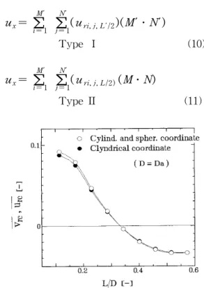
Fig. 10. Correlation of the average radial velocity at center of vessel, v _rc^, and , u _rc, with distance between two impellers, L/D.

Fig. 10에서 이 교반조 중앙의 평균 r - 방향 속도와 임펠러 사이의 거리에 대한 상관관계를 나타냈다.

Fig. 10으로부터 구형조 및 원통조의 차이는 어느 임펠러 사이의 거리에서도 거의 나타나지 않았고, 흐름의 방향이 변하는 임펠러 사이의 거리에서도 서로 일치하고 있는 것을 알았다.

3. 결론

임펠러 및 축 부분은 원통좌표계로 교반조벽 부분은 구좌표계로 수치해석 행하고, 양좌표를 교반조내에서 접합하는 수법을 이용하여 패들 임펠러를 갖춘 구형 교반조내의 유동상태의 수 치해석을 한 결과 다음과 같은 결론을 얻었다.

조 내의 흐름 형태는 의사구형조의 흐름 형태 와 매우 닮고 또 2단 임펠러 흐름의 상태를 표 현하기 위해 지표로 사용한 교반조중앙의 평균 r -방향속도에서도 의사구형조와 같은 모양의 특성을 나타냈다.

이들의 결과로부터 본 연구에서 이용한 수법 으로 경계조건에 의한 원통좌표계에서의 해석, 또는 이좌표계의 접합에 의한 해석이라는 수법 을 이용하여 구형조 내의 유동상태를 수치해석 할 수 있는 것을 알았다.

후 기

본 연구는 상주대학교의 지원에 의해 수행되 었으며 이에 깊은 감사를 드립니다.

사용기호

b = impeller width [m]

b' = apparent impeller width for double- stage impeller [m]

CL = value of f/2∙ReG in laminar flow [-]

Ct = coefficient [-]

Ctr = parameter for transient Reynolds number from laminar to turbulent

flow [-]

D = vessel diameter [m]

d = impeller diameter [m]

D = divergence in Appendix B [-]

Da = apparent vessel diameter for

spherical vessel [m]

Ds = spherical vessel diameter [m]

f = friction factor [-]

Fb = force at vessel bottom [N]

Fs = force at vessel side wall [N]

F R = convection term in Naviour- Stokes Eq. (r-direction) [-]

F S = convection term in Naviour-

Stokes Eq. (θ-direction) [-]

F Z = convection term in Naviour- Stokes Eq. (z-direction) [-]

H = liquid height [m]

L = distance between two impellers for double-stage impeller　　　 　　[m]

M, N, L = number of division [-]

N = rotational speed [s^-1] NP = power number [-]

n_ = number of impeller blade [-]

P = power input [W]

P = pressure 　 　　　　　　　 [N ․ m^-2]

p = dimensionless pressure [-]

R = radial coordinate [m]

r = dimensionless radial coordinate [-]

Re = Reynolds number [-]

Re_d = impeller Reynolds number [-]

Re_G = modified Reynolds number [-]

T = torque [N․ m^-1] T = time [s]

t = dimensionless time [-]

Tb = torque at vessel bottom [N․m]

Ts = torque at vessel side wall [N․m]

Ur = radial velocity in spherical

coordinate [-]

u _{rc r} = average dimensionless radial velocity at center of vessel in spherical coordinate defined Eq.(10) [-]

Uθ = tangential velocity in spherical

coordinate 　　　　 　[m․ s^-1] uθ = dimensionless tangential velocity in spherical coordinate 　 　[-]

Uφ = φ-direction velocity in spherical

coordinate 　　　　 　　 　[m²․s^-1] uφ = dimensionless φ-direction velocity in spherical coordinate [-]

Vγ = radial velocity [m²․s^-1] vγ = dimensionless radial velocity [-]

v _rc = average dimensionless radial velocity at center of vessel defined Eq.(8) [-]

vz = axial velocity [m²․s^-1] uz = dimensionless axial velocity [-]

Vθ =tangential velocity [m²․s^-1] vθ𝜃= dimensionless tangential velocity [-]

Z = axial coordinate [m]

z = dimensionless axial coordinate [-]

α = ratio of torque at bottom wall to

that at side　 　[-]

β = correction factor 　 　[-]

γ = parameter [-]

ε = perturbation in Appendix C [-]

η = correction factor 　　　　　　[-]

θ =tangential coordinate [rad]

μ = fluid viscosity [Pa․s]

ν = kinematic viscosity [m²․s^-1] ρ = fluid density [kg․m^-3]

τ_γθ |w = shear stress at vessel side wall [Pa]

τz θ |w = shear stress at vessel bottom [Pa]

φ = angle in spherical coordinate [rad]

ω = angular velocity [rad․s^-1]

Subscripts w = value at vessel wall

1 = value of single-stage paddle

2 = value of double-stage paddle

calc = calculated value from numerical result equa = calculated value from experimental equation

Superscripts

' = coordinates system fixed on vessel

* = dimensionless

참 고 문 헌

1) Hiraoka, S., Yamada, I. and Mizoguchi, K. : J. Chem. Eng. Japan, 11, 487 (1978).

2) Hiraoka, S., Yamada, I., Aragaki, T., Nishiki, H., sato, A. and Takagi, T. : J.

Chem. Eng. Japen, 21, 79 (1998).

3) Hirt. C. W., Nichols, B. D. and Romero, N. C. : "SOLA" ; LA-5852(1975).

4) Ohta, M., Murakami, M., Arai, K. and Saite, S. : J. Chem. Eng. Japan, 18.

81 (1985).

5) Placek, J. and Tavlarides, L. L. : AIChE Journal, 31, 1113 (1985).

6) Placek, J., Tavlarides, L. L. and Smith, G. W. : AIChE Journal, 32,

1771(1986).

7) Takahashi, S., Chida, T. and Tadaki, T. : Kagaku Kougaku Ronbunshu, 2, 428(1976).

(2007년 9월 29일 접수, 2007년 11월 23일 채택)