A Study on Visual Feedback Control of Industrial Articulated Robot
심병균1*, 이우송2, 박인만3, 황원준3, 최영식4
Byoung-Kyun Shim1*, Woo-Song Lee2, In-Man Park3, Won-Jun hwang3, Young-Sik Choi4
<Abstract>
This paper proposes a new approach to the designed of visual feedback control system based on visual servoing method. The main focus of this paper is presented how it is effective to use many features for improving the accuracy of the visual feedback control of industrial articulated robot for assembling and inspection of parts.
Some rank conditions, which relate the image Jacobian, and the control performance are derived. It is also proven that the accuracy is improved by increasing the number of features. The effectiveness of redundant features is verified by the real time experiments on a SCARA type robot(FARA) made in samsung electronics company.
Keywords : Visual Feedback Control, Visual Servoing, Articulated Robot Arm
1*정회원, 교신저자, 경남대학교 첨단공학과, E-mail:[email protected]
2정회원, 성산암데코 연구소장, 工博
3정회원, 경남대학교 첨단공학과
4정회원, 영남이공대학교 건축과 교수, 工博
1*Corresponding Author, Dept. of Advanced Engineering, Kyungnam University.
2Director, R&D Center, SungSanamdeco Co. Ltd., Ph. D.
3Dept. of Advanced Engineering, Kyungnam University.
4Prof., Department of Architecture, Yeungnam College of Science & Technology, Ph. D.
1. Introduction
There are mainly two ways to put the visual feedback into practice. One is called look-and-move and the other is visual servoing. Visual feedback is the fusion of results from many elemental areas including high-speed image processing, kinematics, dynamics, control theory, and real-time computing.
In the conventional works, some researchers have presented methods to control the manipulator position with respect to the object or to track the feature points on an object using a hand eye system as the application of visual servoing.1) These methods maintain or accomplish a desired
relative position between the camera and the object by monitoring feature points on the object from the camera. However, these have been all done by the hand eye system with monocular visions and it is necessary to compensate for the loss of information because the original three-dimensional information of the scene is reduced to two-dimension information on the image. For instance, we must add information of the three-dimension distance between the feature point and the camera in advance or use a model of object stored in the memory.2)∼3)
This paper presents a method to solve this problem by using a vision. The use of binocular vision can lead to an exact image Jacobian not only at around a desired location
but also at the other locations. The suggested technique places a robot manipulator to the desired location without giving such prior knowledge as the relative distance to the desired location or the model of an object even if the initial positioning error is large.
This paper deals with modeling of high performance vision and how to generate the visual feedback commands. The performance of the proposed visual feedback system was evaluated by the simulations and experiments and obtained results were compared with the conventional case for a SCARA type robot.
2. Visual Feedback Control
Visual servo systems typically use one of two camera configurations: end-effector mounted, or fixed in the workspace.
The first, often called an eye-in-hand configuration, has the camera mounted on the robot's end-effector. Here, there exists a known, often constant, relationship between the pose of the camera(s) and the pose of the end-effector.
We define the frame of a hand-eye system with the stereo vision and use a standard model of the stereo camera whose optical axes are set parallel each other and perpendicular to the baseline. The focal points of two cameras are apart at distance on the baseline and the origin of the camera frame
is located at the center of these cameras.4)An image plane is orthogonal to the optical axis and apart at distance from the focal point of a camera and the origins of frame of the left and right images,
and
, arelocated at the intersecting point of the two optical axes and the image planes. The origin of the world frame
is located at a certain point in the world.5)∼6)Now let and be the projections onto the left and right images of
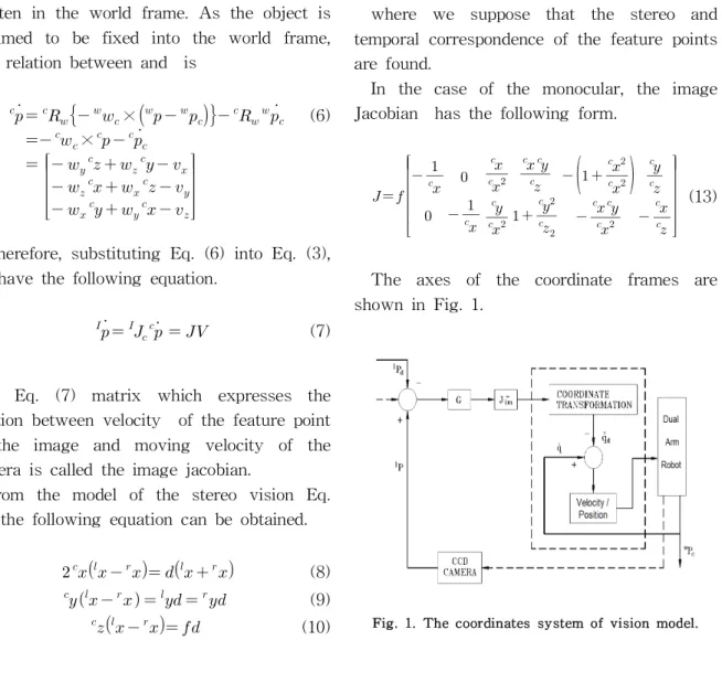
a point in the environment, which is expressed as in the camera frame. Then the following equation is obtained(see Fig. 1).
(1-a)
(1-b)
(1-c)
(1-d)
Suppose that the stereo correspondence of feature points between the left and right images is found. In the visual servoing, we need to know the precise relation between the moving velocity of camera and the velocity of feature points in the image, because we generate a feedback command of the manipulator based on the velocity of feature points in the image.7)
This relation can be expressed in a matrix form which is called the image Jacobian. Let us consider feature points ⋯
on the object and the coordinates in the left and right images are and
, respectively. Also define the current location of the feature points in the image as
⋯ (2)
where each element is expressed with respect to the virtual image frame
.First, to make it simple, let us consider a case when the number of the feature points is one. The relation between the velocity of feature point in image and the velocity of camera frame is given as
(3)
where is the Jacobian matrix which relates the two frames. Now let the
translational velocity components of camera be , , and the rotational velocity components be , , then we can express the camera velocity as
(4)Then the velocity of the feature point seen from the camera frame can be written
(5)
where is the rotation matrix from the camera frame to the world frame and is the location of the origin of the camera frame written in the world frame. As the object is assumed to be fixed into the world frame, The relation between and is
×
×
(6)
Therefore, substituting Eq. (6) into Eq. (3), we have the following equation.
(7)
In Eq. (7) matrix which expresses the relation between velocity of the feature point in the image and moving velocity of the camera is called the image jacobian.
From the model of the stereo vision Eq.
(1), the following equation can be obtained.
(8) (9)
(10)Above discussion is based on the case of one feature point. In practical situation, however, the visual feedback is realized by using plural feature points. When we use feature points, image Jacobian are given from the coordinates of feature points in the image. By combining them, we express the image Jacobian as.
⋯ (11)
Then, it is possible to express the relation of the moving velocity of the camera and the velocity of the feature points even in the case of plural feature points, that is,
(12)
where we suppose that the stereo and temporal correspondence of the feature points are found.
In the case of the monocular, the image Jacobian has the following form.
(13)The axes of the coordinate frames are shown in Fig. 1.
Fig. 1. The coordinates system of vision model.
We now introduce the positional vector of the feature point in the image of monocular vision using the symbol. This is the projection of the point expressed as in the camera frame into the image frame of the monocular vision, and has the following relation.
(14-a)
(14-b)
Substituting Eq.s (14-a) and (14-b) into Eq. (13) yields another expression of the image Jacobian for the monocular vision.
(15)A disparity which corresponds to the depth of the feature point, is included in in the case of the stereo vision, but s-term expressed in the camera frame is included in in the case of the monocular vision.
In the visual servoing, the manipulator is controlled so that the feature points in the image reach their respective desired locations.
We define an error function between the current location of the feature points in image
and the desired location as
(16)where is a matrix which stabilizes the system. Then the feedback law is defined as following equation
(17)
where corresponds to a feedback gain.
To realize the visual servoing, we must choose so that convergence is satisfied
with the error system can be satisfied with
(18)
We use pseudo-inverse matrix of the image Jacobian for to make
positive and not to make an input extremely large, that is,
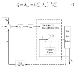
(19)Fig. 2. Block diagram of visual feedback system
Therefore, the feedback command is given as
(20)Fig. 2 shows a block diagram of the control scheme described by Eq. (20). Note that the feedback command is sent to the robot controller and both the transformation of to the desired velocity of each joint angle and its velocity servo are accomplished in the robot controller as show in Fig. 2.
Furthermore, as is a × matrix and pseudo-inverse matrix is a × matrix,
a feedback command Eq. (20) of 6 degrees of freedom is obtained.
3. Experiment and Results
We have compared the visual feedback using the monocular vision with that using the stereo vision by the experiment. Fig. 3 represents the experimental equipment set-up.
In Fig. 3 two DSP vision boards were used, which had been made Samsung Electronics Company in Korea based-on the TMS320C31chips.
In the experiment, feature points of an object are the four corners of a square whose side dimension is . In the same condition, we used four feature point seven In the stereo vision. Parameters used the focal length, , baseline , sampling time of , gain , desired location , desired orientation In Euler angle , initial error in the translation and in the orientation.
Fig. 3. The experimental equipment set-up
We select the four corners of a rectangle whose size is × as the feature points and set the translational error as
and the other values are the same as before.
The error between the desired location and the current location of the feature points in cases of the monocular and stereo visions are shown in Fig. 4.
Next, we will show the results for the change of the way to choose the feature points and set the initial error image.
Two images were taken and transformed to the binary images in the real time and in parallel by two image input devices and the coordinate of the gravitational center of each feature point was calculated in parallel by two transporters. We gave the stereo correspondence of the feature point in the first sampling. However, the stereo and temporal correspondence of the feature points in the succeeding sampling was found automatically by searching a nearby area where there were the feature points in the previous sampling frame. The coordinates of the feature points were sent to a transporter for motion control and it calculated a feedback command for the robot. The result was sent to the robot controller by using RS-232C, and the robot was controlled by a velocity servo system in the controller.
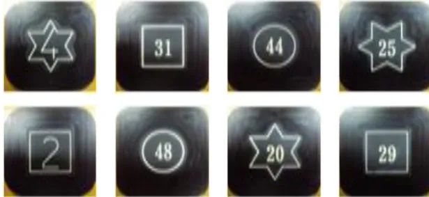
Fig. 4. The parts of diverse shapes used on experiment of visual feedback control
● : Start Point, ◌ : Goal Point (a) Left image
● : Start Point, ◌ : Goal Point (b) Right image
Fig. 5. Trajectories of the feature point on the image(Stereo)
(a) Monocular
(b) Stereo
Fig. 6. Positional error in and axes (simulation)
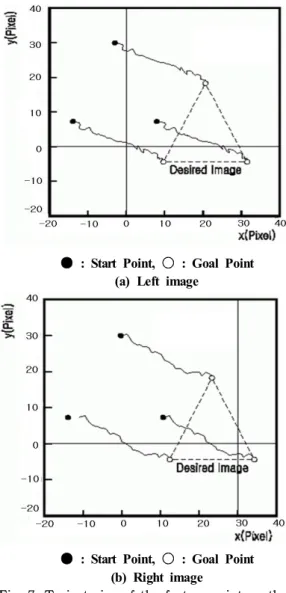
● : Start Point, ◌ : Goal Point (a) Left image
● : Start Point, ◌ : Goal Point (b) Right image
Fig. 7. Trajectories of the feature point on the image
(a) Left image
(b) Right image Fig. 8. Position error in and axes
The sampling period of visual feedback was about . Details were for taking a stereo image, about for calculating the coordinates of the feature points, for calculating feedback command, about for communicating with the robot controller. If we send a feedback input to the robot controller without using RS-232C, the faster visual feedback can be realized. The desired location was
and the desired orientation in Euler angle, degree and the initial error was for translation. The other parameters were the same as in the simulation. Fig. 4 Shows the parts of diverse shapes used on experiment of visual feedback control. And Fig. 5 Shows trajectories of the feature point on the image(Stereo). Fig. 5(a) shows the results about right image, Fig. 5(b) shows the results about left image. Fig. 6 Shows the position error in x and y axes by simulation test. Fig. 6(a) is the results of monocular vision, and Fig. 6(b) is the results of stereo vision. Fig. 7 shows the result of trajectory tracking of the feature point on the image.
Fig. 7(a) is the experiment results about left image, Fig. 7(b) is the experiment results about right image. The error of current and desired location of the feature points are
shown in Fig. 8 From these experimental results, we can see that the manipulator converges toward a desired location even if the calibration is not precise.
4. Conclusion
In this papers it has been proposed a new technique of visual feedback control with the vision to control the position and orientation of an SCARA type robot(FARA) with respect to diverse shaped an object. The suggested technique places a robot manipulator to the desired location without giving such prior knowledge as the relative distance to the desired location or the model of an object even if the initial positioning error is large.
By using the proposed vision method, the image Jacobian can be calculated at any position. Therefore neither shape information nor desired distance of the target object is required. Also we showed the stability of visual feedback was illustrated even when the initial error is large.
REFERENCES
1) Weiss, L. E., Sanderson, A. C., and Neuman, C. P., “Dynamic sensor-based control of robots with visual feedback,”
IEEE Journal of Robotics and Automation, pp. 404-417. (1987)
2) Hashimoto, K., Kimoto, T. Edbine, T., and Kimura, H., “Manipulator control with image-based visual servo,” In Proceedings of IEEE International Conference on Robotics and Automation, pp. 2267-2272.
(1991)
3) Hashimoto, K., Edbine, T., and Kimura, H.,
“Dynamic visual feedback control for a hand-eye manipulator,” In Proceedings of the IEEE/RSJ International Conference on Intelligent Robots and Systems, pp.1863-1868. (1992)
4) G. Hager, S.Hutchinson, and P. I. Corke.“A tutorial on visual servo control,” IEEE Trans. Robotics & Automation, Vol. 12, No. 5, pp. 651-670. (1996)
5) Allen, P. K., Toshimi, B., Timcenko, A.,
“Real Time Visual Servoing,” In Proceeding of the IEEE International Conference on Robotics and Automation, pp. 851-856. (1991)
6) Chaumette, F., Rives, P., and Espiau, B.,
“Positioning of a robot with respoect to an object, tracking it and estimating its velocity by visual servoing,” In Proceedings of the IEEE International Conference on Robotics and Automation, pp. 2248-2253. (1991)
7) Bernard, E., Francois, C., and Patrick, R.,
“A new approach to visual servoing in robotics,” IEEE Transactions on Robotics and Automation, pp. 313-326. (1992)
(접수:2014.01.15, 수정:2014.02.19, 게재확정:2014.02.21)